
迁移学习(图像分类)
在本教程中,您将学习如何使用迁移学习训练卷积神经网络以进行图像分类。您可以在 cs231n 上阅读有关迁移学习的更多信息。
本文主要目的是教会你如何自己搭建分类模型,耐心看完,相信会有很大收获。废话不多说,直切主题…
首先们要知道深度学习大都包含了下面几个方面:
1.加载(处理)数据
2.网络搭建
3.损失函数(模型优化)
4 模型训练和保存
把握好这些主要内容和流程,基本上对分类模型就大致有了个概念。
1.数据加载及处理
我们今天要解决的问题是训练一个模型来对蚂蚁和蜜蜂进行分类。我们有大约120张蚂蚁和蜜蜂的训练图像。每个类有 75 个验证图像。通常,这是一个非常小的数据集,如果从头开始训练,则可以对其进行概括。由于我们使用的是迁移学习,我们应该能够很好地泛化。 加载数据代码部分:
data_transforms = {
    'train': transforms.Compose([
        transforms.RandomResizedCrop(224),
        transforms.RandomHorizontalFlip(),
        transforms.ToTensor(),
        transforms.Normalize([0.485, 0.456, 0.406], [0.229, 0.224, 0.225])
    ]),
    'val': transforms.Compose([
        transforms.Resize(256),
        transforms.CenterCrop(224),
        transforms.ToTensor(),
        transforms.Normalize([0.485, 0.456, 0.406], [0.229, 0.224, 0.225])
    ]),
}

data_dir = 'data/hymenoptera_data'
image_datasets = {x: datasets.ImageFolder(os.path.join(data_dir, x),
                                          data_transforms[x])
                  for x in ['train', 'val']}
dataloaders = {x: torch.utils.data.DataLoader(image_datasets[x], batch_size=4,
                                             shuffle=True, num_workers=4)
              for x in ['train', 'val']}
dataset_sizes = {x: len(image_datasets[x]) for x in ['train', 'val']}
class_names = image_datasets['train'].classes

device = torch.device("cuda:0" if torch.cuda.is_available() else "cpu")
- 1
- 2
- 3
- 4
- 5
- 6
- 7
- 8
- 9
- 10
- 11
- 12
- 13
- 14
- 15
- 16
- 17
- 18
- 19
- 20
- 21
- 22
- 23
- 24
- 25
- 26
- 27
其中:
data_dir = 'data/hymenoptera_data'
- 1
在训练你自己的数据的时候,你需要改为自己的数据路径,并且你需要把你的分类数据按照下面示例进行放置。
假设你要进行猫和狗分类,你需要如下:

并且把每一个种类都分为训练集(train)和验证集(val)如下:
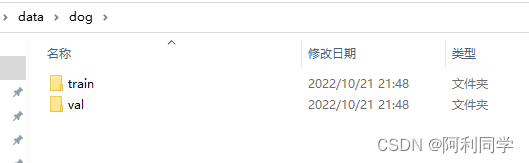
猫的数据也同上进行放置,一般train里面的数据要远多于val文件夹。
本文的数据集可视化图像和代码如下:
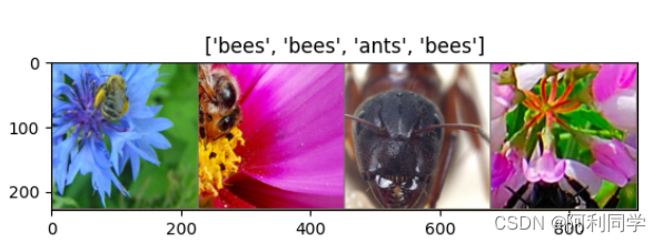
可视化代码:
def imshow(inp, title=None):
    """Imshow for Tensor."""
    inp = inp.numpy().transpose((1, 2, 0))
    mean = np.array([0.485, 0.456, 0.406])
    std = np.array([0.229, 0.224, 0.225])
    inp = std * inp + mean
    inp = np.clip(inp, 0, 1)
    plt.imshow(inp)
    if title is not None:
        plt.title(title)
    plt.pause(0.001)  # pause a bit so that plots are updated


# Get a batch of training data
inputs, classes = next(iter(dataloaders['train']))

# Make a grid from batch
out = torchvision.utils.make_grid(inputs)

imshow(out, title=[class_names[x] for x in classes])
- 1
- 2
- 3
- 4
- 5
- 6
- 7
- 8
- 9
- 10
- 11
- 12
- 13
- 14
- 15
- 16
- 17
- 18
- 19
- 20
模型训练
训练模型的代码示例如下所示:
def train_model(model, criterion, optimizer, scheduler, num_epochs=25):
    since = time.time()

    best_model_wts = copy.deepcopy(model.state_dict())
    best_acc = 0.0

    for epoch in range(num_epochs):
        print(f'Epoch {epoch}/{num_epochs - 1}')
        print('-' * 10)

        # Each epoch has a training and validation phase
        for phase in ['train', 'val']:
            if phase == 'train':
                model.train()  # Set model to training mode
            else:
                model.eval()   # Set model to evaluate mode

            running_loss = 0.0
            running_corrects = 0

            # Iterate over data.
            for inputs, labels in dataloaders[phase]:
                inputs = inputs.to(device)
                labels = labels.to(device)

                # zero the parameter gradients
                optimizer.zero_grad()

                # forward
                # track history if only in train
                with torch.set_grad_enabled(phase == 'train'):
                    outputs = model(inputs)
                    _, preds = torch.max(outputs, 1)
                    loss = criterion(outputs, labels)

                    # backward + optimize only if in training phase
                    if phase == 'train':
                        loss.backward()
                        optimizer.step()

                # statistics
                running_loss += loss.item() * inputs.size(0)


            print(f'{phase} Loss: {epoch_loss:.4f} Acc: {epoch_acc:.4f}')

            # deep copy the model

    print(f'Training complete in {time_elapsed // 60:.0f}m {time_elapsed % 60:.0f}s')
    print(f'Best val Acc: {best_acc:4f}')

    # load best model weights
    model.load_state_dict(best_model_wts)
    return model
- 1
- 2
- 3
- 4
- 5
- 6
- 7
- 8
- 9
- 10
- 11
- 12
- 13
- 14
- 15
- 16
- 17
- 18
- 19
- 20
- 21
- 22
- 23
- 24
- 25
- 26
- 27
- 28
- 29
- 30
- 31
- 32
- 33
- 34
- 35
- 36
- 37
- 38
- 39
- 40
- 41
- 42
- 43
- 44
- 45
- 46
- 47
- 48
- 49
- 50
- 51
- 52
- 53
- 54
- 55
需要你重点关注的是下面这部分代码,我们知道深度学习要学习的目标是缩小给的标签与模型训练值的差距,这里你要是训练狗和猫两类,那么这两类就是dog和cat。loss是重点,该函数通过预测与真实值的做差来使得模型学习我们希望他学习的参数。
特别注意的是.to(device)是GPU加速使用。在模型预测时则不需要使用GPU,就这样模型出来一个值与真实标签值做差的过程中训练了一个良好的分类效果。
 for inputs, labels in dataloaders[phase]:
                inputs = inputs.to(device)
                labels = labels.to(device)

                # zero the parameter gradients
                optimizer.zero_grad()

                # forward
                # track history if only in train
                with torch.set_grad_enabled(phase == 'train'):
                    outputs = model(inputs)
                    _, preds = torch.max(outputs, 1)
                    loss = criterion(outputs, labels)
- 1
- 2
- 3
- 4
- 5
- 6
- 7
- 8
- 9
- 10
- 11
- 12
- 13
网络搭建
有的小伙伴会有疑惑,怎么先模型训练后网络搭建了,其实不是哈,上面只是训练的一个类,下面才是实例化。因为是迁移学习嘛,而且pytorch内置了许多网络供我们选择,因此,此处省去了许多网络搭建,也就是卷积层的搭建过程。此举,意在让我们更快实现分类的目的,而不是过多的重复已有的工作。
model_conv = torchvision.models.resnet18(pretrained=True)
for param in model_conv.parameters():
    param.requires_grad = False

# Parameters of newly constructed modules have requires_grad=True by default
num_ftrs = model_conv.fc.in_features
model_conv.fc = nn.Linear(num_ftrs, 2)

model_conv = model_conv.to(device)

criterion = nn.CrossEntropyLoss()

# Observe that only parameters of final layer are being optimized as
# opposed to before.
optimizer_conv = optim.SGD(model_conv.fc.parameters(), lr=0.001, momentum=0.9)

# Decay LR by a factor of 0.1 every 7 epochs
exp_lr_scheduler = lr_scheduler.StepLR(optimizer_conv, step_size=7, gamma=0.1)
- 1
- 2
- 3
- 4
- 5
- 6
- 7
- 8
- 9
- 10
- 11
- 12
- 13
- 14
- 15
- 16
- 17
- 18
可以看到:
model_conv = torchvision.models.resnet18(pretrained=True)
- 1
此模型采用了resnet18网络,大家都知道这个残差网络具有很好的训练效果,而我们只是一行代码就使用了该网络,可见pytorh的方便之处。
odel_conv.fc = nn.Linear(num_ftrs, 2)
- 1
如果你要进行多类的分类任务,那么你除了在数据集进行变化之外,还需要将上面2这个数字改为 你分类的类别量。
criterion = nn.CrossEntropyLoss()
- 1
- 2
并且这里运用了交叉熵损失函数进行费分类任务,可见损失函数也无需我们进行过多书写,也给我们内置好了函数。
上面说到了上面进行了数据集训练类的书写,下面实例化就完成了类的调用,
model_ft = train_model(model_ft, criterion, optimizer_ft, exp_lr_scheduler,
                       num_epochs=25)
- 1
- 2
为了训练精确,你需要更改 num_epochs=25这里的参数,以及增加你的数据集数量。在我的博客也将写道如何获取想要的数据集。
到此就完成了对图像二分类任务的实现。
本次图像分类任务的精确度较好,由以下看出:
Training complete in 1m 11s
Best val Acc: 0.921569
- 1
- 2
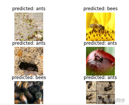
图像二分类任务精度达92%,就问你喜不喜欢。
下面的结果,也证实了准确率:
分类结果
模型保存
模型保存就不再赘述啦,可以私信本人获取,单张图像预测的代码也可以找我!
你要的整体代码如下:
from __future__ import print_function, division

import torch
import torch.nn as nn
import torch.optim as optim
from torch.optim import lr_scheduler
import torch.backends.cudnn as cudnn
import numpy as np
import torchvision
from torchvision import datasets, models, transforms
import matplotlib.pyplot as plt
import time
import os
import copy

cudnn.benchmark = True
plt.ion()   # interactive mode

######################################################################
# Load Data
# ---------
#

data_transforms = {
    'train': transforms.Compose([
        transforms.RandomResizedCrop(224),
        transforms.RandomHorizontalFlip(),
        transforms.ToTensor(),
        transforms.Normalize([0.485, 0.456, 0.406], [0.229, 0.224, 0.225])
    ]),
    'val': transforms.Compose([
        transforms.Resize(256),
        transforms.CenterCrop(224),
        transforms.ToTensor(),
        transforms.Normalize([0.485, 0.456, 0.406], [0.229, 0.224, 0.225])
    ]),
}

data_dir = 'data/hymenoptera_data'
image_datasets = {x: datasets.ImageFolder(os.path.join(data_dir, x),
                                          data_transforms[x])
                  for x in ['train', 'val']}
dataloaders = {x: torch.utils.data.DataLoader(image_datasets[x], batch_size=4,
                                             shuffle=True, num_workers=4)
              for x in ['train', 'val']}
dataset_sizes = {x: len(image_datasets[x]) for x in ['train', 'val']}
class_names = image_datasets['train'].classes

device = torch.device("cuda:0" if torch.cuda.is_available() else "cpu")

######################################################################
# Visualize a few images
# ^^^^^^^^^^^^^^^^^^^^^^
# Let's visualize a few training images so as to understand the data
# augmentations.

def imshow(inp, title=None):
    """Imshow for Tensor."""
    inp = inp.numpy().transpose((1, 2, 0))
    mean = np.array([0.485, 0.456, 0.406])
    std = np.array([0.229, 0.224, 0.225])
    inp = std * inp + mean
    inp = np.clip(inp, 0, 1)
    plt.imshow(inp)
    if title is not None:
        plt.title(title)
    plt.pause(0.001)  # pause a bit so that plots are updated


# Get a batch of training data
inputs, classes = next(iter)

# Make a grid from batch
out = torchvision.utils.make_grid(inputs)

imshow(out, title=[class_names[x] for x in classes])


######################################################################
# Training the model
# ------------------
#
# Now, let's write a general function to train a model. Here, we will
# illustrate:
#
# -  Scheduling the learning rate
# -  Saving the best model
#
# In the following, parameter ``scheduler`` is an LR scheduler object from
# ``torch.optim.lr_scheduler``.


def train_model(model, criterion, optimizer, scheduler, num_epochs=25):
    since = time.time()

    best_model_wts = copy.deepcopy(model.state_dict())
    best_acc = 0.0

    for epoch in range(num_epochs):
        print(f'Epoch {epoch}/{num_epochs - 1}')
        print('-' * 10)

        # Each epoch has a training and validation phase
        for phase in ['train', 'val']:
            if phase == 'train':
                model.train()  # Set model to training mode
            else:
                model.eval()   # Set model to evaluate mode

            running_loss = 0.0
            running_corrects = 0

            # Iterate over data.
            for inputs, labels in dataloaders[phase]:
                inputs = inputs.to(device)
                labels = labels.to(device)

                # zero the parameter gradients
                optimizer.zero_grad()

                # forward
                # track history if only in train
                with torch.set_grad_enabled(phase == 'train'):
                    outputs = model(inputs)
                    _, preds = torch.max(outputs, 1)
                    loss = criterion(outputs, labels)

                    # backward + optimize only if in training phase
                    if phase == 'train':
                        loss.backward()
                        optimizer.step()

                # statistics
                running_loss += loss.item() * inputs.size(0)
                running_corrects += torch.sum(preds == labels.data)
            if phase == 'train':
                scheduler.step()

            epoch_loss = running_loss / dataset_sizes[phase]
            epoch_acc = running_corrects.double() / dataset_sizes[phase]

            print(f'{phase} Loss: {epoch_loss:.4f} Acc: {epoch_acc:.4f}')

            # deep copy the model
            if phase == 'val' and epoch_acc > best_acc:
                best_acc = epoch_acc
                best_model_wts = copy.deepcopy(model.state_dict())

        print()

    time_elapsed = time.time() - since
    print(f'Training complete in {time_elapsed // 60:.0f}m {time_elapsed % 60:.0f}s')
    print(f'Best val Acc: {best_acc:4f}')

    # load best model weights
    model.load_state_dict(best_model_wts)
    return model


######################################################################
# Visualizing the model predictions
# ^^^^^^^^^^^^^^^^^^^^^^^^^^^^^^^^^
#
# Generic function to display predictions for a few images
#

def visualize_model(model, num_images=6):
    was_training = model.training
    model.eval()
    images_so_far = 0
    fig = plt.figure()

    with torch.no_grad():
        for i, (inputs, labels) in enumerate(dataloaders['val']):
            inputs = inputs.to(device)
            labels = labels.to(device)

            outputs = model(inputs)
            _, preds = torch.max(outputs, 1)

            for j in range(inputs.size()[0]):
                images_so_far += 1
                ax = plt.subplot(num_images//2, 2, images_so_far)
                ax.axis('off')
                ax.set_title(f'predicted: {class_names[preds[j]]}')
                imshow(inputs.cpu().data[j])

                if images_so_far == num_images:
                    model.train(mode=was_training)
                    return
        model.train(mode=was_training)

######################################################################
# Finetuning the convnet
# ----------------------
#
# Load a pretrained model and reset final fully connected layer.
#

model_ft = models.resnet18(pretrained=True)
num_ftrs = model_ft.fc.in_features
# Here the size of each output sample is set to 2.
# Alternatively, it can be generalized to nn.Linear(num_ftrs, len(class_names)).
model_ft.fc = nn.Linear(num_ftrs, 2)

model_ft = model_ft.to(device)

criterion = nn.CrossEntropyLoss()

# Observe that all parameters are being optimized
optimizer_ft = optim.SGD(model_ft.parameters(), lr=0.001, momentum=0.9)

# Decay LR by a factor of 0.1 every 7 epochs
exp_lr_scheduler = lr_scheduler.StepLR(optimizer_ft, step_size=7, gamma=0.1)

######################################################################
# Train and evaluate
# ^^^^^^^^^^^^^^^^^^
#
# It should take around 15-25 min on CPU. On GPU though, it takes less than a
# minute.
#

model_ft = train_model(model_ft, criterion, optimizer_ft, exp_lr_scheduler,
                       num_epochs=25)

######################################################################
#

visualize_model(model_ft)


######################################################################
# ConvNet as fixed feature extractor
# ----------------------------------
#
# Here, we need to freeze all the network except the final layer. We need
# to set ``requires_grad = False`` to freeze the parameters so that the
# gradients are not computed in ``backward()``.
#
# You can read more about this in the documentation
# `here `__.
#

model_conv = torchvision.models.resnet18(pretrained=True)
for param in model_conv.parameters():
    param.requires_grad = False

# Parameters of newly constructed modules have requires_grad=True by default
num_ftrs = model_conv.fc.in_features
model_conv.fc = nn.Linear(num_ftrs, 2)

model_conv = model_conv.to(device)

criterion = nn.CrossEntropyLoss()

# Observe that only parameters of final layer are being optimized as
# opposed to before.
optimizer_conv = optim.SGD(model_conv.fc.parameters(), lr=0.001, momentum=0.9)

# Decay LR by a factor of 0.1 every 7 epochs
exp_lr_scheduler = lr_scheduler.StepLR(optimizer_conv, step_size=7, gamma=0.1)


######################################################################
# Train and evaluate
# ^^^^^^^^^^^^^^^^^^
#
# On CPU this will take about half the time compared to previous scenario.
# This is expected as gradients don't need to be computed for most of the
# network. However, forward does need to be computed.
#

model_conv = train_model(model_conv, criterion, optimizer_conv,
                         exp_lr_scheduler, num_epochs=25)

######################################################################
#

visualize_model(model_conv)

plt.ioff()
plt.show()
- 1
- 2
- 3
- 4
- 5
- 6
- 7
- 8
- 9
- 10
- 11
- 12
- 13
- 14
- 15
- 16
- 17
- 18
- 19
- 20
- 21
- 22
- 23
- 24
- 25
- 26
- 27
- 28
- 29
- 30
- 31
- 32
- 33
- 34
- 35
- 36
- 37
- 38
- 39
- 40
- 41
- 42
- 43
- 44
- 45
- 46
- 47
- 48
- 49
- 50
- 51
- 52
- 53
- 54
- 55
- 56
- 57
- 58
- 59
- 60
- 61
- 62
- 63
- 64
- 65
- 66
- 67
- 68
- 69
- 70
- 71
- 72
- 73
- 74
- 75
- 76
- 77
- 78
- 79
- 80
- 81
- 82
- 83
- 84
- 85
- 86
- 87
- 88
- 89
- 90
- 91
- 92
- 93
- 94
- 95
- 96
- 97
- 98
- 99
- 100
- 101
- 102
- 103
- 104
- 105
- 106
- 107
- 108
- 109
- 110
- 111
- 112
- 113
- 114
- 115
- 116
- 117
- 118
- 119
- 120
- 121
- 122
- 123
- 124
- 125
- 126
- 127
- 128
- 129
- 130
- 131
- 132
- 133
- 134
- 135
- 136
- 137
- 138
- 139
- 140
- 141
- 142
- 143
- 144
- 145
- 146
- 147
- 148
- 149
- 150
- 151
- 152
- 153
- 154
- 155
- 156
- 157
- 158
- 159
- 160
- 161
- 162
- 163
- 164
- 165
- 166
- 167
- 168
- 169
- 170
- 171
- 172
- 173
- 174
- 175
- 176
- 177
- 178
- 179
- 180
- 181
- 182
- 183
- 184
- 185
- 186
- 187
- 188
- 189
- 190
- 191
- 192
- 193
- 194
- 195
- 196
- 197
- 198
- 199
- 200
- 201
- 202
- 203
- 204
- 205
- 206
- 207
- 208
- 209
- 210
- 211
- 212
- 213
- 214
- 215
- 216
- 217
- 218
- 219
- 220
- 221
- 222
- 223
- 224
- 225
- 226
- 227
- 228
- 229
- 230
- 231
- 232
- 233
- 234
- 235
- 236
- 237
- 238
- 239
- 240
- 241
- 242
- 243
- 244
- 245
- 246
- 247
- 248
- 249
- 250
- 251
- 252
- 253
- 254
- 255
- 256
- 257
- 258
- 259
- 260
- 261
- 262
- 263
- 264
- 265
- 266
- 267
- 268
- 269
- 270
- 271
- 272
- 273
- 274
- 275
- 276
- 277
- 278
- 279
- 280
- 281
- 282
- 283
如果对你有用,还请三连支持下哦。有什么需要帮助的,可以私信,会及时回复的!!

 QQ名片
QQ名片

评论记录:
回复评论: