
目录
6.干涉图堆栈处理(interferogramStack):
ISCE
SBAS处理流程可以参考博主
【时序InSAR开源软件】用isce2(stackSentinel.py)+mintpy进行哨兵一号SBAS小基线集InSAR时序处理全流程-CSDN博客
【INSAR形变监测】SENTINEL-1 TOPS INSAR全流程 (ISCE2+MINTPY)_sentienl-1 形变处理-CSDN博客
ISCE主要是使用stackSentinel.py生成干涉图
源码:isce2/contrib/stack/topsStack/stackSentinel.py at main · isce-framework/isce2 · GitHub
stackSentinel.py输入输出为:
输入数据:SLC、DEM、Orbits数据
输出数据:一系列可运行文件,每个运行文件实际上有几个相互独立的命令,每个运行文件的配置文件包括执行特定命令/函数的处理选项。
stackSentinel.py
stackSentinel.py使用示例
- # interferogram workflow with 2 nearest neighbor connections (default coregistration is NESD):
- stackSentinel.py -s../SLC/ -d ../../MexicoCity/demLat_N18_N20_Lon_W100_W097.dem.wgs84 -b '19 20 -99.5 -98.5' -a ../../AuxDir/ -o ../../Orbits -c 2
-
- # interferogram workflow with all possible interferograms and coregistration with only geometry:
- stackSentinel.py -s../SLC/ -d ../../MexicoCity/demLat_N18_N20_Lon_W100_W097.dem.wgs84 -b '19 20 -99.5 -98.5' -a ../../AuxDir/ -o ../../Orbits -C geometry -c all
-
- # correlation workflow with all possible correlation pairs and coregistration with geometry:
- stackSentinel.py -s../SLC/ -d ../../MexicoCity/demLat_N18_N20_Lon_W100_W097.dem.wgs84 -b '19 20 -99.5 -98.5' -a ../../AuxDir/ -o ../../Orbits -C geometry -c all -W correlation
-
- # slc workflow that produces a coregistered stack of SLCs
- stackSentinel.py -s../SLC/ -d ../../MexicoCity/demLat_N18_N20_Lon_W100_W097.dem.wgs84 -b '19 20 -99.5 -98.5' -a ../../AuxDir/ -o ../../Orbits -C NESD -W slc
stackSentinel.py参数列表
- | 参数 | 短选项 | 长选项 | 类型 | 是否必需 | 默认值 | 选项 | 含义 |
- |--|--|--|--|--|--|--|
- | display_help | -H | --hh | 无 | 否 | 无 | 无 | 显示详细帮助信息,调用 customArgparseAction 打印 helpstr 并退出程序 |
- | slc_directory | -s | --slc_directory | str | 是 | 无 | 无 | 包含所有 Sentinel SLC 的目录 |
- | orbit_directory | -o | --orbit_directory | str | 是 | 无 | 无 | 包含所有轨道数据的目录 |
- | aux_directory | -a | --aux_directory | str | 是 | 无 | 无 | 包含所有辅助文件的目录 |
- | working_directory | -w | --working_directory | str | 否 | ./ | 无 | 工作目录 |
- | dem | -d | --dem | str | 是 | 无 | 无 | DEM 文件的路径 |
- | polarization | -p | --polarization | str | 否 | vv | 无 | SAR 数据的极化方式 |
- | workflow | -W | --workflow | str | 否 | interferogram | slc, correlation, interferogram, offset | InSAR 处理的工作流 |
- | swath_num | -n | --swath_num | str | 否 | 1 2 3 | 无 | 要处理的条带列表 |
- | bbox | -b | --bbox | str | 否 | 无 | 无 | 经纬度边界(SNWE),示例:'19 20 -99.5 -98.5' |
- | exclude_dates | -x | --exclude_dates | str | 否 | 无 | 无 | 要排除处理的日期列表,示例:'20141007,20141031' |
- | include_dates | -i | --include_dates | str | 否 | 无 | 无 | 要包含处理的日期列表,示例:'20141007,20141031' |
- | start_date | --start_date | 无 | str | 否 | 无 | 无 | 堆栈处理的开始日期,格式应为 YYYY-MM-DD,如 2015-01-23 |
- | stop_date | --stop_date | 无 | str | 否 | 无 | 无 | 堆栈处理的结束日期,格式应为 YYYY-MM-DD,如 2017-02-26 |
- | coregistration | -C | --coregistration | str | 否 | NESD | geometry, NESD | 配准选项 |
- | reference_date | -m | --reference_date | str | 否 | 无 | 无 | 参考采集的目录 |
- | snr_misreg_threshold | --snr_misreg_threshold | 无 | str | 否 | 10 | 无 | 使用互相关估计距离失配准的 SNR 阈值 |
- | esd_coherence_threshold | -e | --esd_coherence_threshold | str | 否 | 0.85 | 无 | 使用增强谱分集估计方位失配准的相干阈值 |
- | num_overlap_connections | -O | --num_overlap_connections | str | 否 | 3 | 无 | 用于 NESD 计算(方位偏移失配准)的每个日期和后续日期之间重叠干涉图的数量 |
- | num_connections | -c | --num_connections | str | 否 | 1 | 无 | 每个日期和后续日期之间干涉图的数量 |
- | azimuth_looks | -z | --azimuth_looks | str | 否 | 3 | 无 | 干涉图多视处理时的方位视数 |
- | range_looks | -r | --range_looks | str | 否 | 9 | 无 | 干涉图多视处理时的距离视数 |
- | filter_strength | -f | --filter_strength | str | 否 | 0.5 | 无 | 干涉图滤波的强度 |
- | unw_method | -u | --unw_method | str | 否 | snaphu | icu, snaphu | 解缠方法 |
- | rmFilter | --rmFilter | 无 | bool | 否 | False | 无 | 是否生成一个额外的去除滤波效果的解缠文件 |
- | param_ion | --param_ion | 无 | str | 否 | 无 | 无 | 电离层估计参数文件,若提供将进行电离层估计 |
- | num_connections_ion | --num_connections_ion | 无 | str | 否 | 3 | 无 | 用于电离层估计的每个日期和后续日期之间干涉图的数量 |
- | useGPU | -useGPU | --useGPU | bool | 否 | False | 无 | 当可用时允许程序使用 GPU |
- | num_process | --num_proc | --num_process | int | 否 | 1 | 无 | 每个运行文件中并行运行的任务数量 |
- | num_process4topo | --num_proc4topo | --num_process4topo | int | 否 | 1 | 无 | 并行进程的数量(仅针对地形) |
- | text_cmd | -t | --text_cmd | str | 否 | 无 | 无 | 要添加到每个运行文件每行开头的文本命令 |
- | virtual_merge | -V | --virtual_merge | str | 否 | 无 | True, False | 对合并的 SLC 和几何文件使用虚拟文件,不同工作流有不同默认值 |

其中比较重要的
-s:slc(single look complex)影像所在目录。
-d表示包含影像范围的DEM文件(WGS84),可利用dem.py命令线上下载。
-a为S1-A的的辅助文件目录,因为S1-A的SAR影像可能由不同版本的设备处理仪器(IPF)获得,而S1-B则不需要
-o为S1轨道文件的目录,缺失的文件将自动下载
-b为研究区经纬度范围
-c为SAR影像连接数,确定每景影像与其相邻日期最近的影像生成干涉图的数目,取决于时间基线,对S1而言一般取3
-u为解缠算法,一般选snaphu
-n为SAR影像的subswath的编号,从左到右为1,2,3
-f为干涉影像的滤波强度
-z为方位向的视数
-r为距离向视数,S1的SAR影像的分辨率为5 m * 20 m(距离*方位),视数越小则干涉影像目标点数(或者像元)越多,处理越费时,但是形变细节保留更多。
--reference_date为影像的参考日期。
执行stackSentinel.py命令后会在当前目录生成一系列文件和文件夹,在runfile文件夹下有16个python脚本文件,分别代表干涉处理的步骤,依次运行脚本则得到一堆干涉影像。
注意:使用stackSentinel.py后可能会生成11个run文件,这个是由于stackSentinel.py参数不同导致的
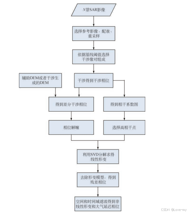
ISCE处理流程
run_01_unpack_topo_reference:
用于配置和执行解包堆栈参考SLC的操作。它会调用unpackStackReferenceSLC方法,从safe_dict中获取相关信息,对参考Sentinel - 1 SLC数据进行解包,将数据从原始的SAFE文件格式转换为适合后续处理的格式。
run_02_unpack_secondary_slc:
负责配置和执行解包辅助SLC的任务。通过调用unpackSecondarysSLC方法,使用stackReferenceDate、secondaryDates和safe_dict中的信息,对辅助日期对应的Sentinel - 1 SLC数据进行解包处理,同样将数据转换为可进一步处理的格式。
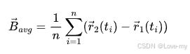
run_03_average_baseline:
用于配置和执行计算平均基线的操作。它调用averageBaseline方法,利用stackReferenceDate和secondaryDates相关数据,计算平均基线。基线信息在后续的干涉测量等处理中非常重要,它反映了不同SLC数据采集时卫星轨道的相对位置关系。
run_04_extract_burst_overlaps:
由于inps.coregistration为NESD且updateStack为False,被生成并用于配置和执行提取突发重叠区域的操作。通过调用extractOverlaps方法,从解包后的SLC数据中确定不同突发之间的重叠区域,这些重叠区域的数据将用于后续的精确配准步骤。
run_05_overlap_geo2rdr:
负责配置和执行将重叠区域从地理坐标转换为距离向坐标并计算偏移量的操作。调用geo2rdr_offset方法,针对secondaryDates对应的SLC数据,在之前提取的重叠区域基础上,进行坐标转换和偏移量计算,为后续的重采样做准备。
run_06_overlap_resample:
用于配置和执行对重叠区域进行带载波重采样的操作。通过调用resample_with_carrier方法,以secondaryDates数据为基础,结合之前计算的偏移量,对重叠区域的数据进行重采样,使不同SLC数据在重叠区域的坐标和分辨率达到一致,便于后续处理。
run_07_pairs_misreg:
如果updateStack为True,配置和执行针对secondaryDates的成对配准误差处理;若updateStack为False,则针对acquisitionDates。通过调用pairs_misregistration方法,利用safe_dict中的数据信息,对每对SLC数据进行配准误差的计算和分析,以确定数据之间的精确差异,为后续的时间序列处理提供基础。
run_08_timeseries_misreg:
用于配置和执行时间序列的配准误差处理。调用timeseries_misregistration方法,综合之前计算的成对配准误差信息,对整个时间序列的SLC数据进行配准误差的进一步分析和处理,以提高数据在时间维度上的一致性和准确性。
run_09_fullBurst_geo2rdr:
负责配置和执行对全突发数据进行从地理坐标到距离向坐标的偏移处理。调用geo2rdr_offset方法,并设置fullBurst='True',对secondaryDates对应的全突发SLC数据进行坐标转换和偏移量计算,与之前重叠区域的处理类似,但针对的是整个突发数据。
run_10_fullBurst_resample:
用于配置和执行对全突发数据进行带载波的重采样操作。调用resample_with_carrier方法,同样设置fullBurst='True',对经过地理到距离向坐标偏移处理后的全突发secondaryDates数据进行重采样,确保全突发数据在坐标和分辨率上的一致性,满足后续处理要求。
run_11_extract_stack_valid_region:
负责配置和执行提取堆栈有效区域的操作。通过调用extractStackValidRegion方法,对经过前面一系列处理后的SLC堆栈数据进行分析,确定数据中的有效区域,排除无效或噪声数据区域,提高后续处理的数据质量。
run_12_merge_reference_secondary_slc:
因为mergeSLC为True,用于配置和执行合并参考SLC和辅助SLC的操作。通过调用mergeReference方法合并参考日期的SLC数据,调用mergeSecondarySLC方法合并secondaryDates对应的辅助SLC数据,并设置virtual = 'False',表示采用实际合并而非虚拟合并的方式,将多个SLC数据合并为一个更便于后续处理的数据集。
run_13_grid_baseline:
负责配置和执行网格化基线的操作。调用gridBaseline方法,使用stackReferenceDate和secondaryDates相关数据,将之前计算的平均基线信息进行网格化处理,将基线数据转换为适合网格化分析和后续应用的格式。
run_14_merge_burst_igram:
配置了合并突发干涉图的操作,接着调用runObj.igram_mergeBurst(acquisitionDates, safe_dict, pairs)方法,将之前生成的突发干涉图进行合并,以得到更完整或适合后续处理的干涉图数据。
run_15_filter_coherence:
用于配置对干涉图相干性进行滤波的操作,然后调用runObj.filter_coherence(pairs)方法,对由pairs确定的干涉图数据进行相干性滤波处理,以提高干涉图的质量和可靠性。
run_16_unwrap:
配置了相位解缠的操作,随后调用runObj.unwrap(pairs)方法,对pairs对应的干涉图数据进行相位解缠处理,将缠绕的相位数据转换为连续的相位值,以便进行后续的变形分析等应用。
stackSentinel.py函数实现
1.边界框处理
generate_geopolygon 函数将用户输入的边界框信息(bbox)转换为 shapely 的 Polygon 对象,使用 shapely.geometry 库,将边界框的经纬度坐标转换为 Point 并创建 Polygon。
2.数据准备与筛选
def get_dates(inps)get_dates 函数负责从 SLC 目录中筛选出所需的 SAFE 文件,根据输入的日期范围(起始日期、结束日期、排除日期、包含日期)、边界框等条件进行筛选。
对于每个 SAFE 文件,创建 sentinelSLC 对象,获取文件的详细信息,包括日期、轨道信息、边界信息(使用 getkmlQUAD 等方法),并存储在 safe_dict 中。
检查 SAFE 文件数量,至少需要两个文件。
确定参考日期 stackReferenceDate 和次要日期列表 secondaryDates。
计算并输出日期列表中所有 SAFE 文件的重叠区域的经纬度范围。
3.相邻日期对的选择
def selectNeighborPairs(dateList, stackReferenceDate, secondaryDates, num_connections, updateStack=False)selectNeighborPairs:对于一般工作流,根据 num_connections 选择相邻日期对。当 num_connections 为具体数字 n 时,从日期列表中选择满足 (dateList[i], dateList[j]) 且 j <= i + n 的日期对;当 num_connections 为 all 时,选择所有可能的相邻日期对。
4.SLC 堆栈处理
- 若不是更新堆栈,先通过 runObj.unpackStackReferenceSLC 解包参考 SLC 的地形信息。
- 解包次要 SLC(runObj.unpackSecondarysSLC)。
- 计算平均基线(runObj.averageBaseline)。
-
- 若使用 NESD 配准:
- 提取重叠区域(runObj.extractOverlaps)。
- 进行几何到距离 - 多普勒(geo2rdr)转换(runObj.geo2rdr_offset)。
-
- 进行重叠区域的重采样(runObj.resample_with_carrier)。
-
- 计算成对的误配准(runObj.pairs_misregistration)。
-
- 计算时间序列误配准(runObj.timeseries_misregistration)。
- 进行全脉冲的几何到距离 - 多普勒转换和重采样。
- 提取堆栈的有效区域(runObj.extractStackValidRegion)。
- 可选择合并参考和次要 SLC 并计算基线网格(runObj.mergeReference 和 runObj.gridBaseline)。
5.相关性堆栈处理(correlationStack):
- 调用 slcStack 进行 SLC 处理。
- 合并参考和次要 SLC(根据 virtual_merge 参数决定是否虚拟合并)。
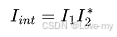
- 生成和合并干涉图的突发(runObj.generate_burstIgram)。对于两个SLC数据I1、I2,干涉图Iint
- 计算相干性并过滤(runObj.filter_coherence)。
6.干涉图堆栈处理(interferogramStack):
- 调用 slcStack 进行 SLC 处理。
- 合并参考和次要 SLC。
- 生成和合并干涉图的突发。
- 过滤相干性。
- 对干涉图进行解缠(runObj.unwrap)。
- 类似于相关性堆栈处理,但增加了解缠步骤。干涉图的相位是缠绕在 [-pi,pi] 范围内的,解缠是将其转换为连续相位,以便更准确地反映地形或地表形变信息,使用 snaphu 或 icu 等方法,基于相位梯度和最小生成树等算法。
解缠:假设缠绕相位为 faiw,解缠的目标是得到连续相位faiu 。基于相邻像素的相位差,满足条件|detfai| ≤pi ,通过区域增长、最小生成树等算法找到最优的解缠路径,使相邻像素的相位差满足此条件,最终将缠绕相位展开为连续相位。
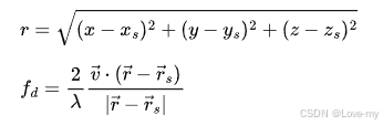
七、偏移堆栈处理(offsetStack):
在 SLC 数据的基础上计算密集偏移,基于互相关函数找到 SLC 数据之间的偏移量,可用于地表位移监测。
八、电离层堆栈处理(ionosphereStack):
利用不同频率子带的干涉图差异来估计电离层延迟,通过一系列处理步骤将电离层延迟信息从干涉图中提取出来。不同频率的信号对电离层延迟的响应不同,通过生成电离层干涉图、解缠和反演等操作得到电离层信息。考虑脉冲特性可提高估计精度,因为不同脉冲受电离层影响不同。
九、状态检查和更新(checkCurrentStatus):
通过文件系统检查和文件命名规则,利用集合操作找出新数据。
Mintpy
主要使用smallbaselineApp.py进行时序分析
源码:MintPy/src/mintpy/smallbaselineApp.py at main · insarlab/MintPy · GitHub
smallbaselineApp.py 实现流程
MintPy的处理流程主要有11步,分别为
(1)加载干涉影像
(2)干涉网络修改
(3)参考点选择
(4)解缠误差改正
(5)网络反演
(6)大气延迟改正
(7)去除相位梯度
(8)地形残余误差改正
(9)剔除噪声SAR影像,确认最佳参考影像
(10)平均LOS速率估计
(11)地理编码。
通过下边这段语句
smallbaselineApp.py -g生成的模板文件,通过执行模板文件可以一次性处理所有步骤
- # vim: set filetype=cfg:
- ##------------------------ smallbaselineApp.cfg ------------------------##
- ########## computing resource configuration
- mintpy.compute.maxMemory = auto #[float > 0.0], auto for 4, max memory to allocate in GB
- ## 分配计算的最大内存,默认为4G
- ## parallel processing with dask
- ## currently apply to steps: invert_network, correct_topography
- ## cluster = none to turn off the parallel computing
- ## numWorker = all to use all of locally available cores (for cluster = local only)
- ## numWorker = 80% to use 80% of locally available cores (for cluster = local only)
- ## config = none to rollback to the default name (same as the cluster type; for cluster != local)
- mintpy.compute.cluster = auto #[local / slurm / pbs / lsf / none], auto for none, cluster type
- ## 集群计算类型
- mintpy.compute.numWorker = auto #[int > 1 / all / num%], auto for 4 (local) or 40 (slurm / pbs / lsf), num of workers
- ## 并行工作的线程数
- mintpy.compute.config = auto #[none / slurm / pbs / lsf ], auto for none (same as cluster), config name
- ## 集群配置名称
-
-
- ########## 1. load_data
- ##---------add attributes manually
- ## MintPy requires attributes listed at: https://mintpy.readthedocs.io/en/latest/api/attributes/
- ## Missing attributes can be added below manually (uncomment #), e.g.
- # ORBIT_DIRECTION = ascending
- # PLATFORM = CSK
- # ...
- ## a. autoPath - automatic path pattern defined in mintpy.defaults.auto_path.AUTO_PATH_*
- ## b. load_data.py -H to check more details and example inputs.
- ## c. compression to save disk usage for ifgramStack.h5 file:
- ## no - save 0% disk usage, fast [default]
- ## lzf - save ~57% disk usage, relative slow
- ## gzip - save ~62% disk usage, very slow [not recommend]
- mintpy.load.processor = auto #[isce, aria, hyp3, gmtsar, snap, gamma, roipac, nisar], auto for isce
- ## 指定处理数据的处理器
- mintpy.load.autoPath = auto #[yes / no], auto for no, use pre-defined auto path
- mintpy.load.updateMode = no #[yes / no], auto for yes, skip re-loading if HDF5 files are complete
- ## 是否在HD5文件完整时跳过加载
- mintpy.load.compression = auto #[gzip / lzf / no], auto for no.
- ## 数据加载压缩方式
- ##---------for ISCE only:
- mintpy.load.metaFile = ../reference/IW*.xml #[path of common metadata file for the stack], i.e.: ./reference/IW1.xml, ./referenceShelve/data.dat
- ## 堆栈公共元数据文件路径
- mintpy.load.baselineDir = ../baselines #[path of the baseline dir], i.e.: ./baselines
- ## 基线目录路径
- ##---------interferogram stack:
- mintpy.load.unwFile = ../merged/interferograms/*/filt_fine.unw #[path pattern of unwrapped interferogram files]
- mintpy.load.corFile = ../merged/interferograms/*/filt_fine.cor #[path pattern of spatial coherence files]
- mintpy.load.connCompFile = ../merged/interferograms/*/filt_fine.unw.conncomp #[path pattern of connected components files], optional but recommended
- mintpy.load.intFile = auto #[path pattern of wrapped interferogram files], optional
- mintpy.load.magFile = auto #[path pattern of interferogram magnitude files], optional
- ##---------ionosphere stack (optional):
- mintpy.load.ionUnwFile = auto #[path pattern of unwrapped interferogram files]
- mintpy.load.ionCorFile = auto #[path pattern of spatial coherence files]
- mintpy.load.ionConnCompFile = auto #[path pattern of connected components files], optional but recommended
- ##---------offset stack (optional):
- mintpy.load.azOffFile = auto #[path pattern of azimuth offset file]
- mintpy.load.rgOffFile = auto #[path pattern of range offset file]
- mintpy.load.azOffStdFile = auto #[path pattern of azimuth offset variance file], optional but recommended
- mintpy.load.rgOffStdFile = auto #[path pattern of range offset variance file], optional but recommended
- mintpy.load.offSnrFile = auto #[path pattern of offset signal-to-noise ratio file], optional
- ##---------geometry:
- mintpy.load.demFile = ../merged/geom_reference/hgt.rdr #[path of DEM file]
- mintpy.load.lookupYFile = ../merged/geom_reference/lat.rdr #[path of latitude /row /y coordinate file], not required for geocoded data
- mintpy.load.lookupXFile = ../merged/geom_reference/lon.rdr #[path of longitude/column/x coordinate file], not required for geocoded data
- mintpy.load.incAngleFile = ../merged/geom_reference/los.rdr #[path of incidence angle file], optional but recommended
- mintpy.load.azAngleFile = ../merged/geom_reference/los.rdr #[path of azimuth angle file], optional
- mintpy.load.shadowMaskFile = ../merged/geom_reference/shadowMask.rdr #[path of shadow mask file], optional but recommended
- mintpy.load.waterMaskFile = auto #[path of water mask file], optional but recommended
- mintpy.load.bperpFile = auto #[path pattern of 2D perpendicular baseline file], optional
- ##---------subset (optional):
- ## if both yx and lalo are specified, use lalo option unless a) no lookup file AND b) dataset is in radar coord
- mintpy.subset.yx = auto #[y0:y1,x0:x1 / no], auto for no
- mintpy.subset.lalo = auto #[S:N,W:E / no], auto for no
-
- #指定经纬范围
- ##---------multilook (optional):
- ## multilook while loading data with the specified method, to reduce dataset size
- ## method - nearest, mean and median methods are applicable to interferogram/ionosphere/offset stack(s), except for:
- ## connected components and all geometry datasets, for which nearest is hardwired.
- ## Use mean / median method with caution! It could smoothen the noise for a better SNR, but it could also smoothen the
- ## unwrapping errors, breaking the integer 2pi relationship, which is used in the unwrapping error correction.
- ## If you really want to increase the SNR, consider re-generate your stack of interferograms with more looks instead.
- mintpy.multilook.method = auto #[nearest, mean, median], auto for nearest - lines/rows skipping approach
- ## 多视处理方式
- mintpy.multilook.ystep = auto #[int >= 1], auto for 1 - no multilooking
- ## y方向多视步长
- mintpy.multilook.xstep = auto #[int >= 1], auto for 1 - no multilooking
-
-
- ########## 2. modify_network
- ## 1) Network modification based on temporal/perpendicular baselines, date, num of connections etc.
- mintpy.network.tempBaseMax = auto #[1-inf, no], auto for no, max temporal baseline in days
- ## 最大时间基线,可以设置一个天数,超过该天数的干涉图将会被排除
- mintpy.network.perpBaseMax = auto #[1-inf, no], auto for no, max perpendicular spatial baseline in meter
- mintpy.network.connNumMax = auto #[1-inf, no], auto for no, max number of neighbors for each acquisition
- mintpy.network.startDate = auto #[20090101 / no], auto for no
- mintpy.network.endDate = auto #[20110101 / no], auto for no
- mintpy.network.excludeDate = auto #[20080520,20090817 / no], auto for no
- mintpy.network.excludeDate12 = auto #[20080520_20090817 / no], auto for no
- mintpy.network.excludeIfgIndex = auto #[1:5,25 / no], auto for no, list of ifg index (start from 0)
- mintpy.network.referenceFile = auto #[date12_list.txt / ifgramStack.h5 / no], auto for no
-
- ## 2) Data-driven network modification
- ## a - Coherence-based network modification = (threshold + MST) by default
- ## reference: Yunjun et al. (2019, section 4.2 and 5.3.1); Chaussard et al. (2015, GRL)
- ## It calculates a average coherence for each interferogram using spatial coherence based on input mask (with AOI)
- ## Then it finds a minimum spanning tree (MST) network with inverse of average coherence as weight (keepMinSpanTree)
- ## Next it excludes interferograms if a) the average coherence < minCoherence AND b) not in the MST network.
- mintpy.network.coherenceBased = auto #[yes / no], auto for no, exclude interferograms with coherence < minCoherence
- mintpy.network.minCoherence = auto #[0.0-1.0], auto for 0.7
-
- ## b - Effective Coherence Ratio network modification = (threshold + MST) by default
- ## reference: Kang et al. (2021, RSE)
- ## It calculates the area ratio of each interferogram that is above a spatial coherence threshold.
- ## This threshold is defined as the spatial coherence of the interferograms within the input mask.
- ## It then finds a minimum spanning tree (MST) network with inverse of the area ratio as weight (keepMinSpanTree)
- ## Next it excludes interferograms if a) the area ratio < minAreaRatio AND b) not in the MST network.
- mintpy.network.areaRatioBased = auto #[yes / no], auto for no, exclude interferograms with area ratio < minAreaRatio
- mintpy.network.minAreaRatio = auto #[0.0-1.0], auto for 0.75
-
- ## Additional common parameters for the 2) data-driven network modification
- mintpy.network.keepMinSpanTree = auto #[yes / no], auto for yes, keep interferograms in Min Span Tree network
- mintpy.network.maskFile = auto #[file name, no], auto for waterMask.h5 or no [if no waterMask.h5 found]
- mintpy.network.aoiYX = auto #[y0:y1,x0:x1 / no], auto for no, area of interest for coherence calculation
- ## 感兴趣的范围(y,x)
- mintpy.network.aoiLALO = auto #[S:N,W:E / no], auto for no - use the whole area
- ## 感兴趣的范围(经纬度)
-
- ########## 3. reference_point
- ## Reference all interferograms to one common point in space
- ## auto - randomly select a pixel with coherence > minCoherence
- ## however, manually specify using prior knowledge of the study area is highly recommended
- ## with the following guideline (section 4.3 in Yunjun et al., 2019):
- ## 1) located in a coherence area, to minimize the decorrelation effect.
- ## 2) not affected by strong atmospheric turbulence, i.e. ionospheric streaks
- ## 3) close to and with similar elevation as the AOI, to minimize the impact of spatially correlated atmospheric delay
- mintpy.reference.yx = auto #[257,151 / auto]
- ## 参考点 y,x的坐标
- mintpy.reference.lalo = auto #[31.8,130.8 / auto]
- ## 参考点经纬度
- mintpy.reference.maskFile = auto #[filename / no], auto for maskConnComp.h5
- ## 参考点选用的掩码文件
- mintpy.reference.coherenceFile = auto #[filename], auto for avgSpatialCoh.h5
- ## 参考点使用的相干性文件
- mintpy.reference.minCoherence = auto #[0.0-1.0], auto for 0.85, minimum coherence for auto method
- ## 自动选择参考点的最小相干性
-
-
- ########## quick_overview
- ## A quick assessment of:
- ## 1) possible groud deformation
- ## using the velocity from the traditional interferogram stacking
- ## reference: Zebker et al. (1997, JGR)
- ## 2) distribution of phase unwrapping error
- ## from the number of interferogram triplets with non-zero integer ambiguity of closue phase
- ## reference: T_int in Yunjun et al. (2019, CAGEO). Related to section 3.2, equation (8-9) and Fig. 3d-e.
- ## 这部分不用配置,主要是对可能的地面变形和相位展开误差分布进行快速评估
-
-
- ########## 4. correct_unwrap_error (optional)
- ## connected components (mintpy.load.connCompFile) are required for this step.
- ## SNAPHU (Chem & Zebker,2001) is currently the only unwrapper that provides connected components as far as we know.
- ## reference: Yunjun et al. (2019, section 3)
- ## supported methods:
- ## a. phase_closure - suitable for highly redundant network
- ## b. bridging - suitable for regions separated by narrow decorrelated features, e.g. rivers, narrow water bodies
- ## c. bridging+phase_closure - recommended when there is a small percentage of errors left after bridging
- mintpy.unwrapError.method = auto #[bridging / phase_closure / bridging+phase_closure / no], auto for no
- ## 展开误差矫正的方法
- mintpy.unwrapError.waterMaskFile = auto #[waterMask.h5 / no], auto for waterMask.h5 or no [if not found]
- mintpy.unwrapError.connCompMinArea = auto #[1-inf], auto for 2.5e3, discard regions smaller than the min size in pixels
-
- ## phase_closure options:
- ## numSample - a region-based strategy is implemented to speedup L1-norm regularized least squares inversion.
- ## Instead of inverting every pixel for the integer ambiguity, a common connected component mask is generated,
- ## for each common conn. comp., numSample pixels are radomly selected for inversion, and the median value of the results
- ## are used for all pixels within this common conn. comp.
- mintpy.unwrapError.numSample = auto #[int>1], auto for 100, number of samples to invert for common conn. comp.
-
- ## bridging options:
- ## ramp - a phase ramp could be estimated based on the largest reliable region, removed from the entire interferogram
- ## before estimating the phase difference between reliable regions and added back after the correction.
- ## bridgePtsRadius - half size of the window used to calculate the median value of phase difference
- mintpy.unwrapError.ramp = auto #[linear / quadratic], auto for no; recommend linear for L-band data
- ## 用于矫正的的相位斜坡类型,L波段推荐linear
- mintpy.unwrapError.bridgePtsRadius = auto #[1-inf], auto for 50, half size of the window around end points
-
- ##解缠误差改正是MIntPy的创新点之一,分别为bridging和phase_closure,前者适用于水体分隔区域,如岛屿等,后者适用于高冗余网络。此步骤可选,建议执行。
- ########## 5. invert_network
- ## Invert network of interferograms into time-series using weighted least square (WLS) estimator.
- ## weighting options for least square inversion [fast option available but not best]:
- ## a. var - use inverse of covariance as weight (Tough et al., 1995; Guarnieri & Tebaldini, 2008) [recommended]
- ## b. fim - use Fisher Information Matrix as weight (Seymour & Cumming, 1994; Samiei-Esfahany et al., 2016).
- ## c. coh - use coherence as weight (Perissin & Wang, 2012)
- ## d. no - uniform weight (Berardino et al., 2002) [fast]
- ## SBAS (Berardino et al., 2002) = minNormVelocity (yes) + weightFunc (no)
- mintpy.networkInversion.weightFunc = auto #[var / fim / coh / no], auto for var
- ## 最小二乘反演的加权函数
- mintpy.networkInversion.waterMaskFile = auto #[filename / no], auto for waterMask.h5 or no [if not found]
- mintpy.networkInversion.minNormVelocity = auto #[yes / no], auto for yes, min-norm deformation velocity / phase
-
- ## mask options for unwrapPhase of each interferogram before inversion (recommend if weightFunct=no):
- ## a. coherence - mask out pixels with spatial coherence < maskThreshold
- ## b. connectComponent - mask out pixels with False/0 value
- ## c. no - no masking [recommended].
- ## d. range/azimuthOffsetStd - mask out pixels with offset std. dev. > maskThreshold [for offset]
- mintpy.networkInversion.maskDataset = auto #[coherence / connectComponent / rangeOffsetStd / azimuthOffsetStd / no], auto for no
- mintpy.networkInversion.maskThreshold = auto #[0-inf], auto for 0.4
- mintpy.networkInversion.minRedundancy = auto #[1-inf], auto for 1.0, min num_ifgram for every SAR acquisition
-
- ## Temporal coherence is calculated and used to generate the mask as the reliability measure
- ## reference: Pepe & Lanari (2006, IEEE-TGRS)
- mintpy.networkInversion.minTempCoh = auto #[0.0-1.0], auto for 0.7, min temporal coherence for mask
- mintpy.networkInversion.minNumPixel = auto #[int > 1], auto for 100, min number of pixels in mask above
- mintpy.networkInversion.shadowMask = auto #[yes / no], auto for yes [if shadowMask is in geometry file] or no.
- ## 是否使用阴影掩码
-
-
- ########## correct_LOD
- ## Local Oscillator Drift (LOD) correction (for Envisat only)
- ## reference: Marinkovic and Larsen (2013, Proc. LPS)
- ## automatically applied to Envisat data (identified via PLATFORM attribute)
- ## and skipped for all the other satellites.
- ## 本地振荡器漂移校正,仅适用于Envisat数据
-
- ########## 6. correct_SET
- ## Solid Earth tides (SET) correction [need to install insarlab/PySolid]
- ## reference: Milbert (2018); Yunjun et al. (2022, IEEE-TGRS)
- mintpy.solidEarthTides = auto #[yes / no], auto for no
- ## 固体地球潮汐校正,需要安装insarlab/PySolid
-
-
- ########## 7. correct_ionosphere (optional but recommended)
- ## correct ionospheric delay [need split spectrum results from ISCE-2 stack processors]
- ## reference:
- ## ISCE-2 topsApp/topsStack: Liang et al. (2019, IEEE-TGRS)
- ## ISCE-2 stripmapApp/stripmapStack: Fattahi et al. (2017, IEEE-TGRS)
- ## ISCE-2 alos2App/alosStack: Liang et al. (2018, IEEE-TGRS)
- mintpy.ionosphericDelay.method = auto #[split_spectrum / no], auto for no
- ## 电离层延迟的方法
- mintpy.ionosphericDelay.excludeDate = auto #[20080520,20090817 / no], auto for no
- mintpy.ionosphericDelay.excludeDate12 = auto #[20080520_20090817 / no], auto for no
-
-
- ########## 8. correct_troposphere (optional but recommended)
- ## correct tropospheric delay using the following methods:
- ## a. height_correlation - correct stratified tropospheric delay (Doin et al., 2009, J Applied Geop)
- ## b. pyaps - use Global Atmospheric Models (GAMs) data (Jolivet et al., 2011; 2014)
- ## ERA5 - ERA5 from ECMWF [need to install PyAPS from GitHub; recommended and turn ON by default]
- ## MERRA - MERRA-2 from NASA [need to install PyAPS from Caltech/EarthDef]
- ## NARR - NARR from NOAA [need to install PyAPS from Caltech/EarthDef; recommended for N America]
- ## c. gacos - use GACOS with the iterative tropospheric decomposition model (Yu et al., 2018, JGR)
- ## need to manually download GACOS products at http://www.gacos.net for all acquisitions before running this step
- mintpy.troposphericDelay.method = no #[pyaps / height_correlation / gacos / no], auto for pyaps
- ## 对流层延迟校正的方法
-
- ## Notes for pyaps:
- ## a. GAM data latency: with the most recent SAR data, there will be GAM data missing, the correction
- ## will be applied to dates with GAM data available and skipped for the others.
- ## b. WEATHER_DIR: if you define an environment variable named WEATHER_DIR to contain the path to a
- ## directory, then MintPy applications will download the GAM files into the indicated directory.
- ## MintPy application will look for the GAM files in the directory before downloading a new one to
- ## prevent downloading multiple copies if you work with different dataset that cover the same date/time.
- mintpy.troposphericDelay.weatherModel = auto #[ERA5 / MERRA / NARR], auto for ERA5
- ## 使用pyaps方法,需要指定要使用的全球大气模型
- mintpy.troposphericDelay.weatherDir = auto #[path2directory], auto for WEATHER_DIR or "./"
- ## 使用pyaps方法,需要指定存储全球大气模型数据的路径
-
- ## Notes for height_correlation:
- ## Extra multilooking is applied to estimate the empirical phase/elevation ratio ONLY.
- ## For an dataset with 5 by 15 looks, looks=8 will generate phase with (5*8) by (15*8) looks
- ## to estimate the empirical parameter; then apply the correction to original phase (with 5 by 15 looks),
- ## if the phase/elevation correlation is larger than minCorrelation.
- mintpy.troposphericDelay.polyOrder = auto #[1 / 2 / 3], auto for 1
- mintpy.troposphericDelay.looks = auto #[1-inf], auto for 8, extra multilooking num
- mintpy.troposphericDelay.minCorrelation = auto #[0.0-1.0], auto for 0
-
- ## Notes for gacos:
- ## Set the path below to directory that contains the downloaded *.ztd* files
- mintpy.troposphericDelay.gacosDir = auto # [path2directory], auto for "./GACOS"
-
-
- ########## 9. deramp (optional)
- ## Estimate and remove a phase ramp for each acquisition based on the reliable pixels.
- ## Recommended for localized deformation signals, i.e. volcanic deformation, landslide and land subsidence, etc.
- ## NOT recommended for long spatial wavelength deformation signals, i.e. co-, post- and inter-seimic deformation.
- mintpy.deramp = linear #[no / linear / quadratic], auto for no - no ramp will be removed
- ## 指定去斜坡处理的方法类型
- mintpy.deramp.maskFile = auto #[filename / no], auto for maskTempCoh.h5, mask file for ramp estimation
- ## 去斜坡处理的掩码文件
-
-
- ########## 10. correct_topography (optional but recommended)
- ## Topographic residual (DEM error) correction
- ## reference: Fattahi and Amelung (2013, IEEE-TGRS)
- ## stepDate - specify stepDate option if you know there are sudden displacement jump in your area,
- ## e.g. volcanic eruption, or earthquake
- ## excludeDate - dates excluded for the error estimation
- ## pixelwiseGeometry - use pixel-wise geometry (incidence angle & slant range distance)
- ## yes - use pixel-wise geometry if they are available [slow; used by default]
- ## no - use the mean geometry [fast]
- mintpy.topographicResidual = auto #[yes / no], auto for yes
- ## 地形残差校正(DEM校正)
- mintpy.topographicResidual.polyOrder = auto #[1-inf], auto for 2, poly order of temporal deformation model
- mintpy.topographicResidual.phaseVelocity = auto #[yes / no], auto for no - use phase velocity for minimization
- mintpy.topographicResidual.stepDate = auto #[20080529,20190704T1733 / no], auto for no, date of step jump
- mintpy.topographicResidual.excludeDate = auto #[20070321 / txtFile / no], auto for exclude_date.txt
- mintpy.topographicResidual.pixelwiseGeometry = auto #[yes / no], auto for yes, use pixel-wise geometry info
-
-
- ########## 11.1 residual_RMS (root mean squares for noise evaluation)
- ## Calculate the Root Mean Square (RMS) of residual phase time-series for each acquisition
- ## reference: Yunjun et al. (2019, section 4.9 and 5.4)
- ## To get rid of long spatial wavelength component, a ramp is removed for each acquisition
- ## Set optimal reference date to date with min RMS
- ## Set exclude dates (outliers) to dates with RMS > cutoff * median RMS (Median Absolute Deviation)
- mintpy.residualRMS.maskFile = auto #[file name / no], auto for maskTempCoh.h5, mask for ramp estimation
- mintpy.residualRMS.deramp = auto #[quadratic / linear / no], auto for quadratic
- ## 计算残差均方根时斜坡的去除类型
- mintpy.residualRMS.cutoff = auto #[0.0-inf], auto for 3
-
- ########## 11.2 reference_date
- ## Reference all time-series to one date in time
- ## reference: Yunjun et al. (2019, section 4.9)
- ## no - do not change the default reference date (1st date)
- mintpy.reference.date = no #[reference_date.txt / 20090214 / no], auto for reference_date.txt
- ## 将所有时间序列参考指定日期
-
-
- ########## 12. velocity
- ## Estimate a suite of time functions [linear velocity by default]
- ## from final displacement file (and from tropospheric delay file if exists)
- mintpy.timeFunc.startDate = auto #[20070101 / no], auto for no
- mintpy.timeFunc.endDate = auto #[20101230 / no], auto for no
- mintpy.timeFunc.excludeDate = auto #[exclude_date.txt / 20080520,20090817 / no], auto for exclude_date.txt
-
- ## Fit a suite of time functions
- ## reference: Hetland et al. (2012, JGR) equation (2-9)
- ## polynomial function is defined by its degree in integer. 1 for linear, 2 for quadratic, etc.
- ## periodic function(s) are defined by a list of periods in decimal years. 1 for annual, 0.5 for semi-annual, etc.
- ## step function(s) are defined by a list of onset times in str in YYYYMMDD(THHMM) format
- ## exp & log function(s) are defined by an onset time followed by an charateristic time in integer days.
- ## Multiple exp and log functions can be overlaied on top of each other, achieved via e.g.:
- ## 20110311,60,120 - two functions sharing the same onset time OR
- ## 20110311,60;20170908,120 - separated by ";"
- mintpy.timeFunc.polynomial = auto #[int >= 0], auto for 1, degree of the polynomial function
- mintpy.timeFunc.periodic = auto #[1,0.5 / list_of_float / no], auto for no, periods in decimal years
- mintpy.timeFunc.stepDate = auto #[20110311,20170908 / 20120928T1733 / no], auto for no, step function(s)
- mintpy.timeFunc.exp = auto #[20110311,60 / 20110311,60,120 / 20110311,60;20170908,120 / no], auto for no
- mintpy.timeFunc.log = auto #[20110311,60 / 20110311,60,120 / 20110311,60;20170908,120 / no], auto for no
-
- ## Uncertainty quantification methods:
- ## a. residue - propagate from fitting residue assuming normal dist. in time (Fattahi & Amelung, 2015, JGR)
- ## b. covariance - propagate from time series (co)variance matrix
- ## c. bootstrap - bootstrapping (independently resampling with replacement; Efron & Tibshirani, 1986, Stat. Sci.)
- mintpy.timeFunc.uncertaintyQuantification = auto #[residue, covariance, bootstrap], auto for residue
- mintpy.timeFunc.timeSeriesCovFile = auto #[filename / no], auto for no, time series covariance file
- mintpy.timeFunc.bootstrapCount = auto #[int>1], auto for 400, number of iterations for bootstrapping
-
-
- ########## 13.1 geocode (post-processing)
- # for input dataset in radar coordinates only
- # commonly used resolution in meters and in degrees (on equator)
- # 100, 90, 60, 50, 40, 30, 20, 10
- # 0.000925926, 0.000833334, 0.000555556, 0.000462963, 0.000370370, 0.000277778, 0.000185185, 0.000092593
- mintpy.geocode = auto #[yes / no], auto for yes
- ## 是否进行地理编码
- mintpy.geocode.SNWE = auto #[-1.2,0.5,-92,-91 / none ], auto for none, output extent in degree
- ## 输出地理范围(经纬度)
- mintpy.geocode.laloStep = auto #[-0.000555556,0.000555556 / None], auto for None, output resolution in degree
- ## 输出分辨率
- mintpy.geocode.interpMethod = auto #[nearest], auto for nearest, interpolation method
- ## 地理编码差值方法
- mintpy.geocode.fillValue = auto #[np.nan, 0, ...], auto for np.nan, fill value for outliers.
- ## 异常值填充值
-
- ########## 13.2 google_earth (post-processing)
- mintpy.save.kmz = auto #[yes / no], auto for yes, save geocoded velocity to Google Earth KMZ file
- ## 是否将地理编码后的速度保存到谷歌地球的KMZ文件
-
- ########## 13.3 hdfeos5 (post-processing)
- mintpy.save.hdfEos5 = auto #[yes / no], auto for no, save time-series to HDF-EOS5 format
- ## 是否将时间序列保存到HD5格式
- mintpy.save.hdfEos5.update = auto #[yes / no], auto for no, put XXXXXXXX as endDate in output filename
- mintpy.save.hdfEos5.subset = auto #[yes / no], auto for no, put subset range info in output filename
-
- ########## 13.4 plot
- # for high-resolution plotting, increase mintpy.plot.maxMemory
- # for fast plotting with more parallelization, decrease mintpy.plot.maxMemory
- mintpy.plot = auto #[yes / no], auto for yes, plot files generated by default processing to pic folder
- mintpy.plot.dpi = auto #[int], auto for 150, number of dots per inch (DPI)
- mintpy.plot.maxMemory = 16 #[float], auto for 4, max memory used by one call of view.py for plotting.
SBAS流程实现
1.配准
SAR单视复数影像的配准主要分为两个步骤: 粗配准和精配准。
(1)粗配准:通常选取参考影像的中心点作为参考点由于参考影像中心点在副影像上有唯一对应点,进而利用参考影像和副影像的卫星轨道参数及 InSAR 成像几何求得参考影像中心点在副影像中的对应点,并把它们作为配准的同名点对。
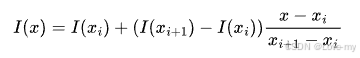
(2)精配准:是在粗配准基础上, 通过同名点坐标或其偏移量建立参考影像到副影像的坐标映射关系, 再利用这个关系对副影像进行坐标变换、 影像插值和重采样。精配准的方法有:相干系数阈值法、 最大频谱法和相位差影像平均波动函数法。
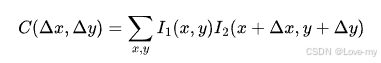
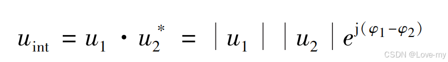
2.干涉图生成
两景配准后每一点数据为:
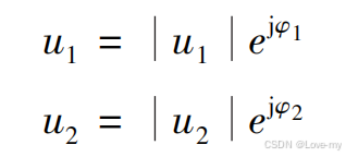
则干涉值为:
3.干涉图滤波
干涉影像的噪声来源主要有时间/空间基线失相干、 热噪声、 数据处理误差 等, 为了减小噪声对后续解缠的影响,需采取滤波的方法对干涉影像进行处理,
针对干涉 SAR 影像中随机噪声的特性,将抑制噪声的方法大体分为两类: 空间域滤波和频率域滤波。
空间域滤波方法主要有: 条纹自适应滤波方法、 多视滤波方法和矢量滤波方法等。
频率域滤波方法主要有: 自适应滤波 (Goldstein 滤 波) 方法、 频谱加权滤波方法、 小波滤波方法等。
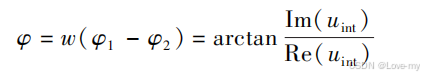
4.相位解缠
给定同一地区的两景 SAR 影像, 经过配准之后,对应像元进行共轭相乘得 到相位差, 并形成干涉图, 但是从干涉图中得到的相位差实际上是主值,即在 ( -π,π)呈周期性变化,为了还原其真实的相位差,必须在主值的基础上加或 减整数倍的相位周期2π,把被卷叠的相位展开,才能顺利地反演出地面目标的高程和形变。
常用的解缠方法(二维相位解缠):
1.Goldstein 枝切法相位解缠
2.最小二乘法相位解缠
5.地理编码
将雷达坐标系下的原始数据通过一定的几何校正方法消除由轨道、 传感器、 地球模型引起的扭曲和畸变,然后变换到某种制图参考系 (地图投影) 中以便于人们对获取的地理信息进行理解和判读,这一过程被称为 SAR 影像的地理编码。
地理编码:影像行列坐标(l,p)->零多普勒时间系统->以地球为原点的三维笛卡尔坐标系(X,Y,Z).
ICA分解
主要参考
1.原文:Independent Component Analysis: A Tutorial Introduction | MIT Press eBooks | IEEE Xplore
2.独立分量分析(Independent Component Analysis) - 知乎
3.独立成分分析(Independent Component Analysis) - 知乎
4.学习笔记 | 独立成分分析(ICA, FastICA)及应用-CSDN博客
5.独立成分分析(ICA)模型推导与代码实践_哔哩哔哩_bilibili
代码实现思路
1.读取数据信息
(1)地理变换信息
栅格行列数、像素大小以及旋转信息,以便为独立成分的生成提供相同信息。
(2)投影信息
2.缺失值处理
使用本行均值填充
3.FastICA
影像数组长这样
评论记录:
回复评论: