这个博客其实从7月2号就开始写了，本以为半个月就能搞出来，结果稀稀拉拉整了1个多月才研究明白（这不给来个三连→_→）。BPU对我来说还是太新鲜了，其中涉及到的相关技术，对我这种小白来说，真的是挑战很大。

我们都知道BPU可以加速深度学习的推理，也非常想掌握这个技术。官方文档及其全面，进而导致我无法快速的上手。如果想熟练掌握BPU开发，需要会使用docker，理解为什么转换模型需要调优（说白了还是我菜?）。

这篇博客，我会一步步引导各位使用BPU，进而递进地掌握如下一些基本技能，比如

• docker基本配置。包含windows下的安装与基本使用
• 在BPU上部署手部关键点检测算法。目的是引导各位如何快速地将caffe模型部署到BPU上。
• 在BPU上部署边缘检测HED算法。Caffe模型中包含自定义层，这又该如何部署呢。
• 在BPU上部署目标跟踪算法。

部署后地模型将会运行在旭日x3开发板上，里面有一块BPU芯片，用于加速深度学习的推理过程。

本博客所介绍的相关软件都放在百度云（提取码：0a09 ）里了。

本部分的相关文档可参考：Horizon AI Toolchain User Guide

一 安装准备

本部分介绍了在使用工具链前必须的环境准备工作，包含开发机部署(个人电脑) 和开发板部署(例如旭日开发板等包含BPU设备) 两个部分。

1.1 开发机部署(个人电脑)

官方的示例教程的开发机都是Linux系统，实际上Windows系统也是可以的。最建议的方式是利用docker，模型转换过程主要还是基于CPU，用不到GPU，所以用docker就够了。

1.1.1 安装docker

考虑到用户多数是基于个人电脑，所以相关环境的配置都是基于Windows的。
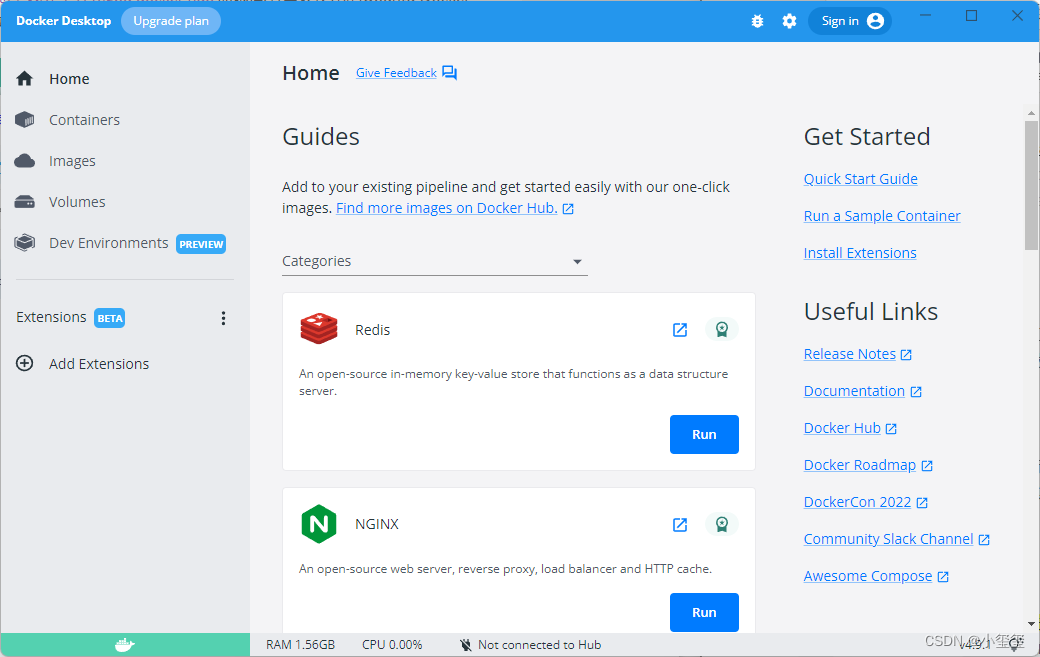
在百度云的软件文件夹里，提供了Docker Desktop Installer.exe安装文件，安装之后，用管理员方式启动得到如下界面。

我们可以从地平线天工开物cpu docker hub获取部署所需要的CentOS Docker镜像。我们使用最新的镜像v1.13.6

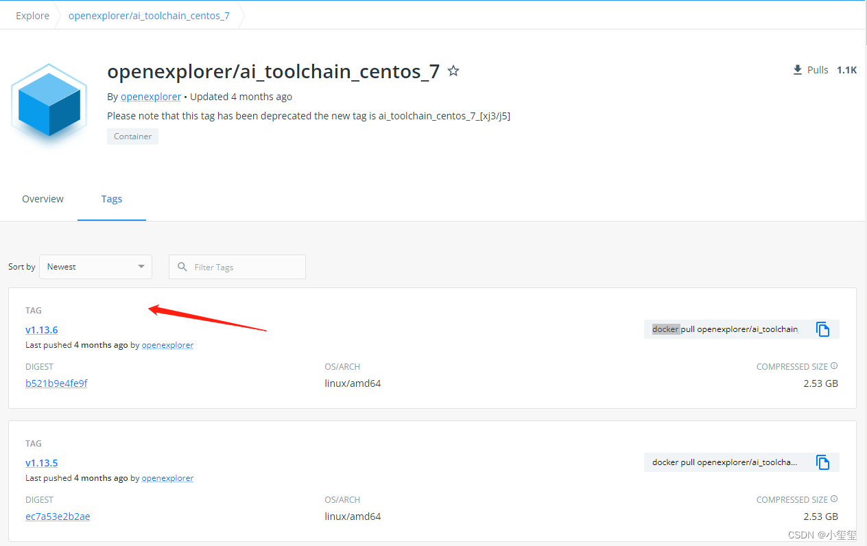
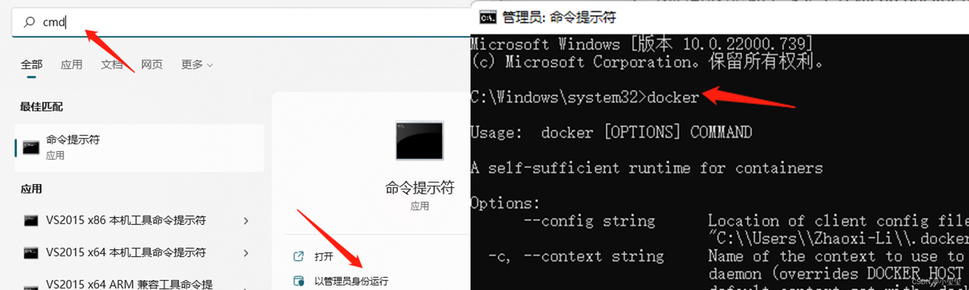
以管理员模式运行CMD，输入docker，可以显示出docker的帮助信息。我们选择最新版本，则在cmd中输入命令docker pull openexplorer/ai_toolchain_centos_7:v1.13.6，之后会自动开始docker的安装。

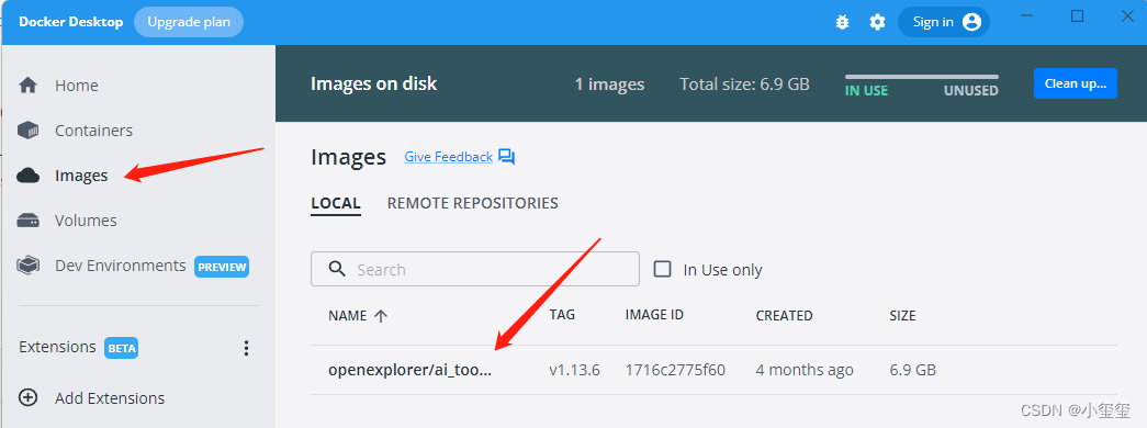
安装成功之后，即可在docker中看到我们成功安装了工具链镜像：

1.1.2 配置天工开物OpenExplorer

OpenExplorer工具包的下载，需要wget支持，wget的下载链接为：GNU Wget for Windows，安装好之后即可在cmd中通过如下命令下载工具包，工具包我也放在百度云中的OpenExplorer文件夹，下载之后要解压这个包。
wget -c ftp://vrftp.horizon.ai/Open_Explorer_gcc_9.3.0/2.2.3/horizon_xj3_open_explorer_v2.2.3_20220617.tar.gz
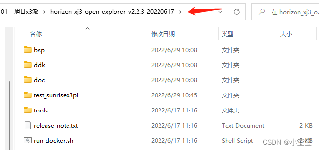
解压后，工具包的内容如下所示，如果需要其他版本的，可以参考官网信息资料下载专区。

docker除了要挂载OpenExplorer工具包，还要挂载数据集文件夹，通过如下指令可以下载官方提供的数据集，或者从百度云的OpenExplorer/dataset文件夹中下载，下载之后记得解压（正常部署的过程用不上这些，先下载下来，说不定以后用到了呢）。

# cifar
wget -c ftp://vrftp.horizon.ai/Open_Explorer/eval_dataset/cifar-10.tar.gz 
# cityscapes
wget -c ftp://vrftp.horizon.ai/Open_Explorer/eval_dataset/cityscapes.tar.gz 
# coco
wget -c ftp://vrftp.horizon.ai/Open_Explorer/eval_dataset/coco.tar.gz 
# imagenet
wget -c ftp://vrftp.horizon.ai/Open_Explorer/eval_dataset/imagenet.tar.gz 
# VOC
wget -c ftp://vrftp.horizon.ai/Open_Explorer/eval_dataset/VOC.tar.gz

• 1
• 2
• 3
• 4
• 5
• 6
• 7
• 8
• 9
• 10

由于我在Windows下解压的，因此部分软连接消失，因此我补充了一些必要的软连接更新

# 重新构建model_zoo软连接
rm /open_explorer/ddk/samples/ai_toolchain/horizon_model_convert_sample/01_common/model_zoo
ln -s /open_explorer/ddk/samples/ai_toolchain/model_zoo /open_explorer/ddk/samples/ai_toolchain/horizon_model_convert_sample/01_common/model_zoo

• 1
• 2
• 3

1.1.3 启动Docker

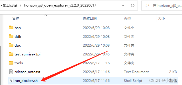
按照教程，启动docker要执行run_docker.sh，本意是想简化操作，但我觉得没啥必要，可以按照本文教程直接配置好指令即可。

在进入docker之前，先记录两个内容：

• 天工开物OpenExplorer根目录：我的环境下是"D:\05 - 项目\01 - 旭日x3派\horizon_xj3_open_explorer_v2.2.3_20220617"，记得加双引号防止出现空格，该目录要挂载在docker中/open_explorer目录下
• dataset根目录：我的环境下是"D:\01 - datasets"，记得加双引号防止出现空格，该目录需要挂载在docker中的/data/horizon_x3/data目录下。
• *辅助文件夹根目录：官方教程其实是没有这个过程的，我把这个挂载在docker里，就是充当个类似U盘的介质。比如在我的环境下是"D:\05 - 项目\01 - 旭日x3派\BPUCodes"，我可以在windows里面往这个文件夹拷贝数据，这些数据就可以在docker中使用，在docker中的路径为/data/horizon_x3/codes。

那么，在cmd（管理员）中输入如下指令即可进入docker（切记要确保刚刚安装的软件docker desktop是开启的）

CMD不支持换行，记得删掉后面的\然后整理为一行

docker run -it --rm \
-v "D:\05 - 项目\01 - 旭日x3派\horizon_xj3_open_explorer_v2.2.3_20220617":/open_explorer \
-v "D:\01 - datasets":/data/horizon_x3/data \
-v "D:\05 - 项目\01 - 旭日x3派\BPUCodes":/data/horizon_x3/codes \
openexplorer/ai_toolchain_centos_7:v1.13.6

• 1
• 2
• 3
• 4
• 5

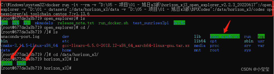
这时候，我们可以看到由命令行挂载的3个目录啦。

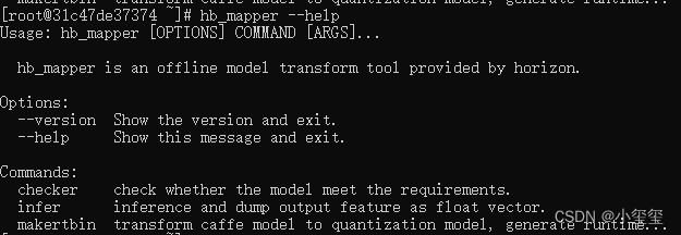
至此，已经成功通过Docker镜像进入了完整的工具链开发环境。 可以键入 hb_mapper --help 命令验证下是否可以正常得到帮助信息，hb_mapper 是工具链的一个常用工具， 在后文的模型转换部分对其有详细介绍。

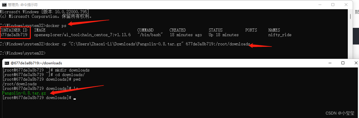
除了通过挂载个额外的文件夹来实现文件的拷贝，还有个方法可以直接将文件拷贝到目标目录。
假如我们要拷贝一个文件"C:\Users\Zhaoxi-Li\Downloads\Pangolin-0.8.tar.gz"到docker中的/root/downloads下（目录要存在哈），那么用管理员权限新开一个cmd，输入docker ps，记录CONTAINER ID，然后按照docker cp 本地文件的路径 container_id:的方式输入docker cp "C:\Users\Zhaoxi-Li\Downloads\Pangolin-0.8.tar.gz" 677de3a8b719:/root/downloads即可完成文件拷贝。

1.2 开发板部署(旭日3派为例)

在使用之前，一定要按照教程多方位玩转“地平线新发布AIoT开发板——旭日X3派(Sunrise x3 Pi)”完成系统的启动。

工具链的部分补充工具未包含在系统镜像中，这些工具已经放置在Open Explorer发布包中。因此在我们刚刚拉取的docker中，输入cd /open_explorer/ddk/package/board/，执行命令bash install.sh 192.168.0.104，其中192.168.0.104为开发板IP地址，可用ifconfig查看。

这个功能主要就是拷贝hrt_bin_dump和hrt_model_exec到开发板，并在开发板的/etc/profile里面添加几个环境，添加内容如下所示。

#Horizon Open Explorer ENV
export PATH=/userdata/.horizon/:/userdata/.horizon/ai_express_webservice_display/sbin/:$PATH
export HORIZON_APP_PATH=/userdata/.horizon/:$HORIZON_APP_PATH
#Horizon Open Explorer ENV

• 1
• 2
• 3
• 4

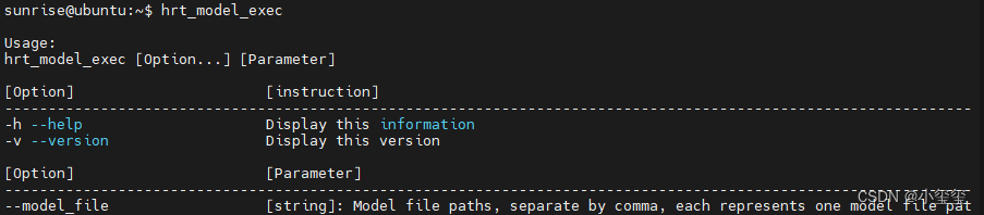
在开发板里输入hrt_model_exec，如果有如下输出，说明开发板部署完成。

二 深度学习模型部署

BPU的工具链是非常长的，在部署先，一定要先理解下每个流程的含义，有个意识，不需要理解原理，只需要理解干了啥。在后面的部署过程中会反过来对着这些流程进行理解。

• 模型准备：支持Caffe模型和ONNX模型，Caffe模型的支持度是最高的。咱们常用的Pytorch模型是可以转为ONNX模型的。实际上，OpenCV内部集成的dnn模块也是以caffe为主的，所以尽管Caffe在学术圈不火了，但它在工业圈一直广泛使用（看来还得继续捡起来继续深读源码）。
• 验证模型：验证模型中所用的层是否可以在BPU中使用。需要利用hb_mapper checker后面跟一堆参数来对模型进行配置。配置信息如下（第一次看到这里的话，不用看配置信息，后面进行模型转化的时候，反过来再看这里）：
  • --model-type：输入的模型类型，onnx或caffe ；
  • --march：芯片类型，这个板子只能填bernoulli2；
  • --proto：若模型为caffe，则填入caffe所需的prototxt文件。onnx模型就不用写这个参数
  • --model：模型文件，caffe就是*****.caffemodel，onnx模型就是****.onnx。
  • --input-shape：模型数据输入的名称和维度，比如输入层名称叫input1，维度为1x3x128x128，那么该参数就可以写为--input-shape input1 1x3x128x128。如果我们的模型有多个输入，比如第二个输入层名称叫input2，维度为1x96x28x28，那么参数设置就写为--input-shape input1 1x3x128x128 --input-shape input2 1x96x28x28。（该参数可选，不写的话程序会自动识别参数，如果指定以指定为主）
  • --output：设置输出日志文件（已经移除，默认存在根目录的hb_mapper_checker.log中）。
  • 注意：如果模型检查不通过，控制台会有明显的ERROR信息，一般都会检查出某些层不支持BPU，这时候可以写个自定义层来解决，后面会提供个例子来展示不通过情况的处理办法。
• 转换模型：模型检查通过之后，就可以通过配置一个yaml文件来将模型文件转为可以在BPU上运行的文件了。这个是整个环节最为困难的一部分，这里我不进行展开讲，后面配置模型时候会详细介绍。
  • --model-type：根据模型类型指定caffe或onnx
  • --config：模型编译的配置文件，内容采用yaml格式，文件名使用.yaml后缀。这里面有30多个参数，初学者
• 模型性能、精度分析与调优。初时BPU的时候都会疑惑，为什么转换模型后精度会有变化?因为模型转换后是由float转为int8计算的，这个过程必有精度损失。如果精度差异较大，就需要按照官方教程进行调优。

本博客的目的是让大家快速部署自己的模型，部署后精度只是有少量损失。关于调优部分，量比较多，会单独再开一个进行详细讲解。

2.1 官方示例：Yolov3部署

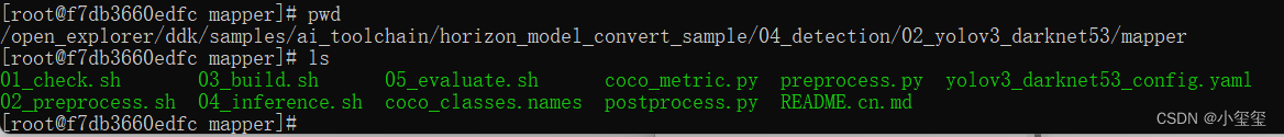
yolov3放置在docker中的/open_explorer/ddk/samples/ai_toolchain/horizon_model_convert_sample/04_detection/02_yolov3_darknet53/mapper路径下，下面先以官方示例进行部署，每一步都进行一个讲解，来初步了解下BPU的相关操作流程。

2.1.1 模型准备

模型所需要的prototxt和caffemodel文件放置在docker中的/open_explorer/ddk/samples/ai_toolchain/model_zoo/mapper/detection/yolov3_darknet53路径下。

2.1.2 验证模型

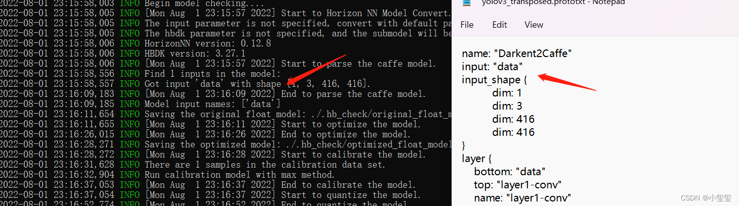
进入路径/open_explorer/ddk/samples/ai_toolchain/horizon_model_convert_sample/04_detection/02_yolov3_darknet53/mapper，输入 ./01_check.sh，遇到下述这些输出，就代表转换完成了。

前面已经介绍了，模型验证需要利用hb_mapper checker后面跟一堆参数来对模型进行配置，下面这些就是 ./01_check.sh的主要内容。

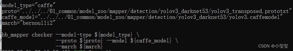
下面带各位来理解这些参数：

• --model-type：我们这些模型是Caffe，所以填caffe
• --march：旭日3派只能填bernoulli2
• --proto：填prototxt文件路径，即../../../01_common/model_zoo/mapper/detection/yolov3_darknet53/yolov3_transposed.prototxt
• --model：填caffemodel文件路径，即../../../01_common/model_zoo/mapper/detection/yolov3_darknet53/yolov3.caffemodel
• --input-shape：这里没有指定，代码可以自动去查找（多输入的话就自己指定吧）。
  

2.1.3 转换模型

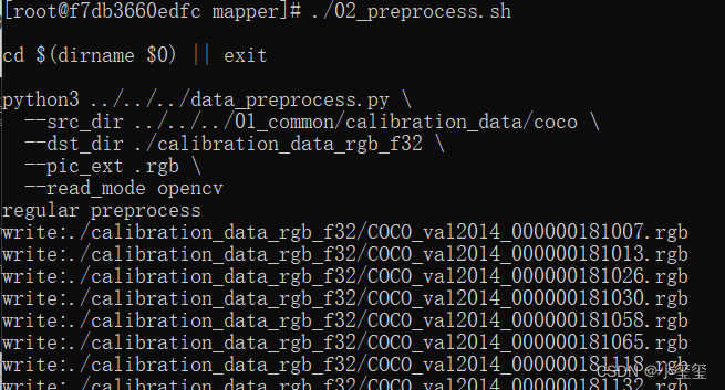
在转换模型之前需要准备校准数据，输入./02_preprocess.sh会自动从docker的open_explorer包中抽取数据。

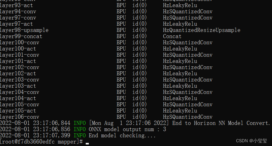
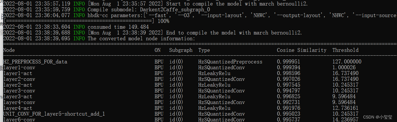
再输入./03_build.sh，输出一大堆的命令行，等待一段时间之后会输出。这里我们可以发现每一层网络都要评估一个相似度。这也是为什么要准备校准数据，因为BPU是INT8计算，所以注定会有精度损失。而且这些误差也是可以传递的，所以到后面精度是越来越低的。如果网络深度过高，也会导致整体精度的下降。

为了更好的理解这些转换流程，我对其中的准备校准数据、模型转换过程进行一个完全解读。

(i) 原理解读：准备校准数据

这个过程调用了脚本./02_preprocess.sh，这个脚本核心调用的是python文件，data_preprocess.py的源码可以自行去查看。

python3 ../../../data_preprocess.py \
  --src_dir ../../../01_common/calibration_data/coco \
  --dst_dir ./calibration_data_rgb_f32 \
  --pic_ext .rgb \
  --read_mode opencv

• 1
• 2
• 3
• 4
• 5

然而data_preprocess.py并不适合初学者进行阅读，因为其兼容了太多东西，很简单的一些功能硬是写复杂了，那么就围绕这个模型，给各位缕缕校准数据到底要准备啥。

首先要搞清楚，我们要准备的校准数据是什么样的： 校准数据要将图像数据按照目标尺寸、目标颜色(rgb or bgr等)、目标排布(CHW or HWC) 进行存储。
那么下面，带着这些问题进行处理，先构建一个基本处理流程：

1. 加载一个文件夹下的所有图像地址信息。图像目录为/open_explorer/ddk/samples/ai_toolchain/horizon_model_convert_sample/01_common/calibration_data/coco
2. 对每个图像按照校准格式进行输出。从prototxt我们知道图像的尺寸为416x416，从./03_build.sh调用的yaml文件可知图像输入格式为rgb，数据排布为CHW
3. 将转换后的图像利用numpy.tofile函数存到目标文件夹下/open_explorer/ddk/samples/ai_toolchain/horizon_model_convert_sample/04_detection/02_yolov3_darknet53/mapper/calibration_data。你在哪转换的，就要在哪个目录存校准数据文件夹calibration_data。

下面，开始写我们自己的Python代码，每个步骤都写了注释，各位可以直接理解。

# prepare_calibration_data.py
import os
import cv2
import numpy as np

src_root = '/open_explorer/ddk/samples/ai_toolchain/horizon_model_convert_sample/01_common/calibration_data/coco'
cal_img_num = 100  # 想要的图像个数
dst_root = '/open_explorer/ddk/samples/ai_toolchain/horizon_model_convert_sample/04_detection/02_yolov3_darknet53/mapper/calibration_data'


## 1. 从原始图像文件夹中获取100个图像作为校准数据
num_count = 0
img_names = []
for src_name in sorted(os.listdir(src_root)):
    if num_count > cal_img_num:
        break
    img_names.append(src_name)
    num_count += 1

# 检查目标文件夹是否存在，如果不存在就创建
if not os.path.exists(dst_root):
    os.system('mkdir {0}'.format(dst_root))

## 2 为每个图像转换
# 参考了OE中/open_explorer/ddk/samples/ai_toolchain/horizon_model_convert_sample/01_common/python/data/下的相关代码
# 转换代码写的很棒，很智能，考虑它并不是官方python包，所以我打算换一种写法

## 2.1 定义图像缩放函数，返回为np.float32
# 图像缩放为目标尺寸(W, H)
# 值得注意的是，缩放时候，长宽等比例缩放，空白的区域填充颜色为pad_value, 默认127
def imequalresize(img, target_size, pad_value=127.):
    target_w, target_h = target_size
    image_h, image_w = img.shape[:2]
    img_channel = 3 if len(img.shape) > 2 else 1

    # 确定缩放尺度，确定最终目标尺寸
    scale = min(target_w * 1.0 / image_w, target_h * 1.0 / image_h)
    new_h, new_w = int(scale * image_h), int(scale * image_w)

    resize_image = cv2.resize(img, (new_w, new_h))

    # 准备待返回图像
    pad_image = np.full(shape=[target_h, target_w, img_channel], fill_value=pad_value)

    # 将图像resize_image放置在pad_image的中间
    dw, dh = (target_w - new_w) // 2, (target_h - new_h) // 2
    pad_image[dh:new_h + dh, dw:new_w + dw, :] = resize_image

    return pad_image

## 2.2 开始转换
for each_imgname in img_names:
    img_path = os.path.join(src_root, each_imgname)

    img = cv2.imread(img_path)  # BRG, HWC
    img = cv2.cvtColor(img, cv2.COLOR_BGR2RGB)  # RGB, HWC
    img = imequalresize(img, (416, 416))
    img = np.transpose(img, (2, 0, 1))  # RGB, CHW

    # 将图像保存到目标文件夹下
    dst_path = os.path.join(dst_root, each_imgname + '.rgbchw')
    print("write:%s" % dst_path)
    # 图像加载默认就是uint8，但是不加这个astype的话转换模型就会出错
    # 转换模型时候，加载进来的数据竟然是float64，不清楚内部是怎么加载的。
    img.astype(np.uint8).tofile(dst_path) 

print('finish')

• 1
• 2
• 3
• 4
• 5
• 6
• 7
• 8
• 9
• 10
• 11
• 12
• 13
• 14
• 15
• 16
• 17
• 18
• 19
• 20
• 21
• 22
• 23
• 24
• 25
• 26
• 27
• 28
• 29
• 30
• 31
• 32
• 33
• 34
• 35
• 36
• 37
• 38
• 39
• 40
• 41
• 42
• 43
• 44
• 45
• 46
• 47
• 48
• 49
• 50
• 51
• 52
• 53
• 54
• 55
• 56
• 57
• 58
• 59
• 60
• 61
• 62
• 63
• 64
• 65
• 66
• 67

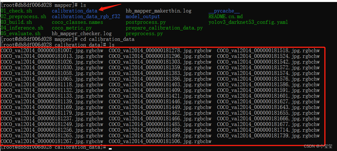
执行这些代码之后，在目录下，就生成了我们的校准数据

(ii) 原理解读：转换配置

模型转换的核心在于配置目标的yaml文件，官方也提供了一个yolov3_darknet53_config.yaml可供用户直接试用，每个参数都给了注释，我能感受到开发者的诚意。然而模型转换的配置文件参数太多，如果想改参数都不知道如何下手。

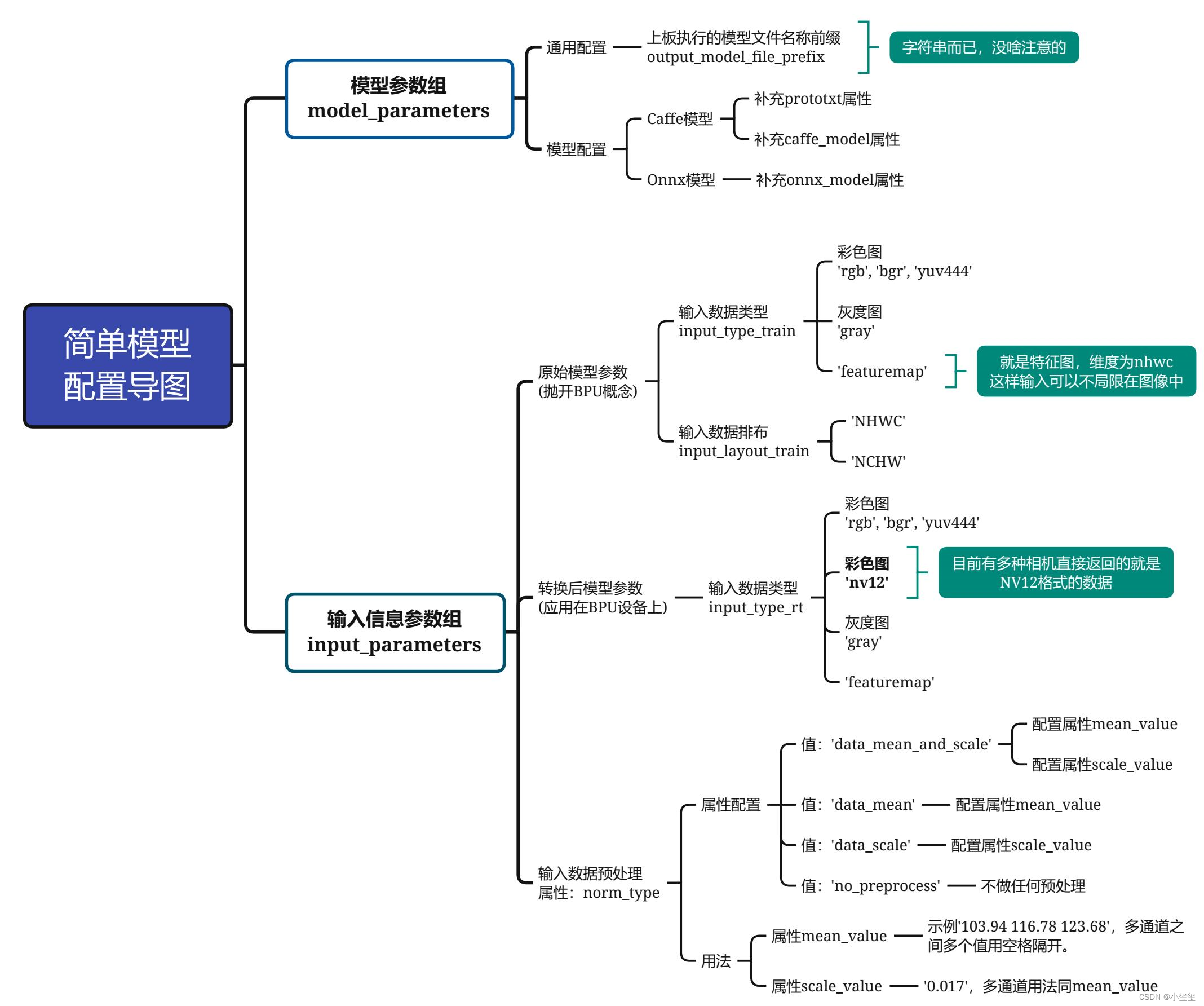
本节目的是引导各位快速上手，因此一些参数我暂时不解释意义，用默认即可。该模板可将待配置的30多个参数压缩到9个参数，方便各位快速的配置简单模型。本yaml模板适用于的模型具有如下属性：

• 无自定义层，换句话说，BPU支持该模型的所有层。
• 输入节点只有1个，且输入是图像。

先复制这个模板到代码根目录，命名为"yolov3_simple.yaml"，然后根据后面的思维导图进行配置具体参数。

model_parameters:
  # [待配置参数]，见思维导图"模型参数组"部分
  prototxt: '***.prototxt'
  caffe_model: '****.caffemodel'
  onnx_model: '****.onnx'
  output_model_file_prefix: 'mobilenetv1'
  
  # 默认参数，暂不需要理解
  march: 'bernoulli2'

input_parameters:
  # [待配置参数]，见思维导图"输入信息参数组/原始模型参数"部分
  input_type_train: 'bgr'
  input_layout_train: 'NCHW'

  # [待配置参数]，见思维导图"输入信息参数组/转换后模型参数"部分
  input_type_rt: 'yuv444'

  # [待配置参数]，见思维导图"输入信息参数组/输入数据预处理"部分
  norm_type: 'data_mean_and_scale'
  mean_value: '103.94 116.78 123.68'
  scale_value: '0.017'
  
  # 默认参数，暂不需要理解
  input_layout_rt: 'NHWC'
  

# 校准参数组，全部默认
calibration_parameters:
  cal_data_dir: './calibration_data'
  calibration_type: 'max'
  max_percentile: 0.9999

# 编译参数组，全部默认
compiler_parameters:
  compile_mode: 'latency'
  optimize_level: 'O3'
  debug: False # 别看官网写的可选，实际上不写这个出bug

• 1
• 2
• 3
• 4
• 5
• 6
• 7
• 8
• 9
• 10
• 11
• 12
• 13
• 14
• 15
• 16
• 17
• 18
• 19
• 20
• 21
• 22
• 23
• 24
• 25
• 26
• 27
• 28
• 29
• 30
• 31
• 32
• 33
• 34
• 35
• 36
• 37
• 38

思维导图如下所示，带着这个图，请各位耐心地跟我一步步配置，仅需要配置9个即可。

• 模型参数组参数model_parameters配置：
  • output_model_file_prefix：给转换后的模型起个名，这里叫做'yolov3_selfyaml'，注意字符串前后都要有个单引号。
  • prototxt：caffe的prototxt，这里为'../../../01_common/model_zoo/mapper/detection/yolov3_darknet53/yolov3_transposed.prototxt'
  • caffe_model：caffe的模型文件，这里为'../../../01_common/model_zoo/mapper/detection/yolov3_darknet53/yolov3.caffemodel'
  • onnx_model：删掉。因为我们用的是Caffe。
• 输入信息组参数配置input_parameters：
  • input_type_train：原始浮点模型的输入数据格式，支持多种图像格式，这里设置为'rgb'（这就是前文校准模型时为什么要将BGR转为RGB）。
  • input_layout_train：从前文的prototxt可以看出，数据输入排布为'NCHW'（所以在模型校准时我们将图像数据由HWC转为CHW）
  • input_type_rt：模型转换后，我们期望输入的图像格式。我们在训练模型和部署模型的时候，图像输入格式是可以变的，NV12是一些相机返回的原始数据格式，作为尝试设置为'nv12'。
  • norm_type：网络不可能拿原始图像数据作为输入的，一般都要进行一个归一化操作。这里用的模型对应的归一化代码为inpBlob = cv2.dnn.blobFromImage(frame, 1.0 / 255, (inWidth, inHeight), (0, 0, 0), swapRB=False, crop=False)，无减均值项，只有尺度项。因此，该属性设置为'data_scale'。
  • mean_value：删掉，因为网络没有均值项。
  • scale_value：尺度为1.0 / 255，因此设置为0.003921568627451

最终，我们的yaml文件内容如下所示：

model_parameters:
  prototxt: '../../../01_common/model_zoo/mapper/detection/yolov3_darknet53/yolov3_transposed.prototxt'
  caffe_model: '../../../01_common/model_zoo/mapper/detection/yolov3_darknet53/yolov3.caffemodel'
  output_model_file_prefix: 'yolov3_selfyaml'
  march: 'bernoulli2'
input_parameters:
  input_type_train: 'rgb'
  input_layout_train: 'NCHW'
  input_type_rt: 'nv12'
  norm_type: 'data_scale'
  scale_value: 0.003921568627451
  input_layout_rt: 'NHWC'
calibration_parameters:
  cal_data_dir: './calibration_data'
  calibration_type: 'max'
  max_percentile: 0.9999
compiler_parameters:
  compile_mode: 'latency'
  optimize_level: 'O3'
  debug: False

• 1
• 2
• 3
• 4
• 5
• 6
• 7
• 8
• 9
• 10
• 11
• 12
• 13
• 14
• 15
• 16
• 17
• 18
• 19
• 20

之后，用我们亲手准备的校准数据和配置的轻量yaml进行模型转换，在控制台输入指令hb_mapper makertbin --config yolov3_simple.yaml --model-type caffe

2.1.4 模型推理

在官方给的demo中，04_inference.sh可以直接调用执行好的模型进行推理，但是为了我觉得这种方案对于未来要如何部署自己的模型是无意义的。因此我阅读了官方推理的demo之后，自己写个完整的推理过程。

模型推理流程主要可以分为以下三个步骤：

• 数据预处理，生成推理所需数据。
• 利用处理好的数据进行模型推理，得到输出
• 将输出转换成最终数据，也就是后处理过程。

使用的测试图像路径为/open_explorer/ddk/samples/ai_toolchain/horizon_model_convert_sample/01_common/test_data/det_images/kite.jpg

在上一节中，模型转换后有三个关键文件：

• yolov3_selfyaml_original_float_model.onnx：图像量化前的模型
• yolov3_selfyaml_quantized_model.onnx：图像量化后的模型
• yolov3_selfyaml.bin：在BPU上用于推理的模型文件，输出结果与yolov3_selfyaml_quantized_model.onnx一致。
• yolov3_selfyaml_optimized_float_model.onnx：这个我不知道干啥用的，搜了一圈也没看到在哪用的 - -||。

下面我给出推理一张图像的相关代码，其中我把图像格式转换，以及yolo后处理的细节封装在一个包里，相关的代码已经放在百度云（提取码：0a09 ）里供大家参考。

下面是inference_model.py的代码细节，在每个关键过程中都给出了相关的注释。
下图是yolov3网络的输出，从代码可以获知模型会输出三层，每层的维度为(1, 13, 13, 255) (1, 26, 26, 255) (1, 52, 52, 255)，对着下图，可以很容易对应的是网络的哪一层。

import numpy as np
import cv2
import os
from horizon_tc_ui import HB_ONNXRuntime
from bputools.format_convert import imequalresize, bgr2nv12_opencv, nv122yuv444
from bputools.yolo_postproc import modelout2predbbox, recover_boxes, nms, draw_bboxs

modelpath_prefix = '/open_explorer/ddk/samples/ai_toolchain/horizon_model_convert_sample'

# img_path 图像完整路径
img_path = os.path.join(modelpath_prefix, '01_common/test_data/det_images/kite.jpg')
# model_path 量化模型完整路径
model_root = os.path.join(modelpath_prefix, '04_detection/02_yolov3_darknet53/mapper/model_output')
model_path = os.path.join(model_root, 'yolov3_selfyaml_quantized_model.onnx')

# 1. 加载模型，获取所需输出HW
sess = HB_ONNXRuntime(model_file=model_path)
sess.set_dim_param(0, 0, '?')
model_h, model_w = sess.get_hw()

# 2 加载图像，根据前面模型，转换后的模型是以NV12作为输入的
# 但在OE验证的时候，需要将图像再由NV12转为YUV444
imgOri = cv2.imread(img_path)
img = imequalresize(imgOri, (model_w, model_h))
nv12 = bgr2nv12_opencv(img)
yuv444 = nv122yuv444(nv12, [model_w, model_h])

# 3 模型推理
input_name = sess.input_names[0]
output_name = sess.output_names
output = sess.run(output_name, {input_name: np.array([yuv444])}, input_offset=128)
print(output_name)
print(output[0].shape, output[1].shape, output[2].shape)
# ['layer82-conv-transposed', 'layer94-conv-transposed', 'layer106-conv-transposed']
# (1, 13, 13, 255) (1, 26, 26, 255) (1, 52, 52, 255)

# 4 检测结果后处理
# 由output恢复416*416模式下的目标框
pred_bbox = modelout2predbbox(output)
# 将目标框恢复到原始分辨率
bboxes = recover_boxes(pred_bbox, (imgOri.shape[0], imgOri.shape[1]),
                       input_shape=(model_h, model_w), score_threshold=0.3)
# 对检测出的框进行非极大值抑制，抑制后得到的框就是最终检测框
nms_bboxes = nms(bboxes, 0.45)
print("detected item num: {0}".format(len(nms_bboxes)))

# 绘制检测框
draw_bboxs(imgOri, nms_bboxes)
cv2.imwrite('detected.png', imgOri)

• 1
• 2
• 3
• 4
• 5
• 6
• 7
• 8
• 9
• 10
• 11
• 12
• 13
• 14
• 15
• 16
• 17
• 18
• 19
• 20
• 21
• 22
• 23
• 24
• 25
• 26
• 27
• 28
• 29
• 30
• 31
• 32
• 33
• 34
• 35
• 36
• 37
• 38
• 39
• 40
• 41
• 42
• 43
• 44
• 45
• 46
• 47
• 48
• 49

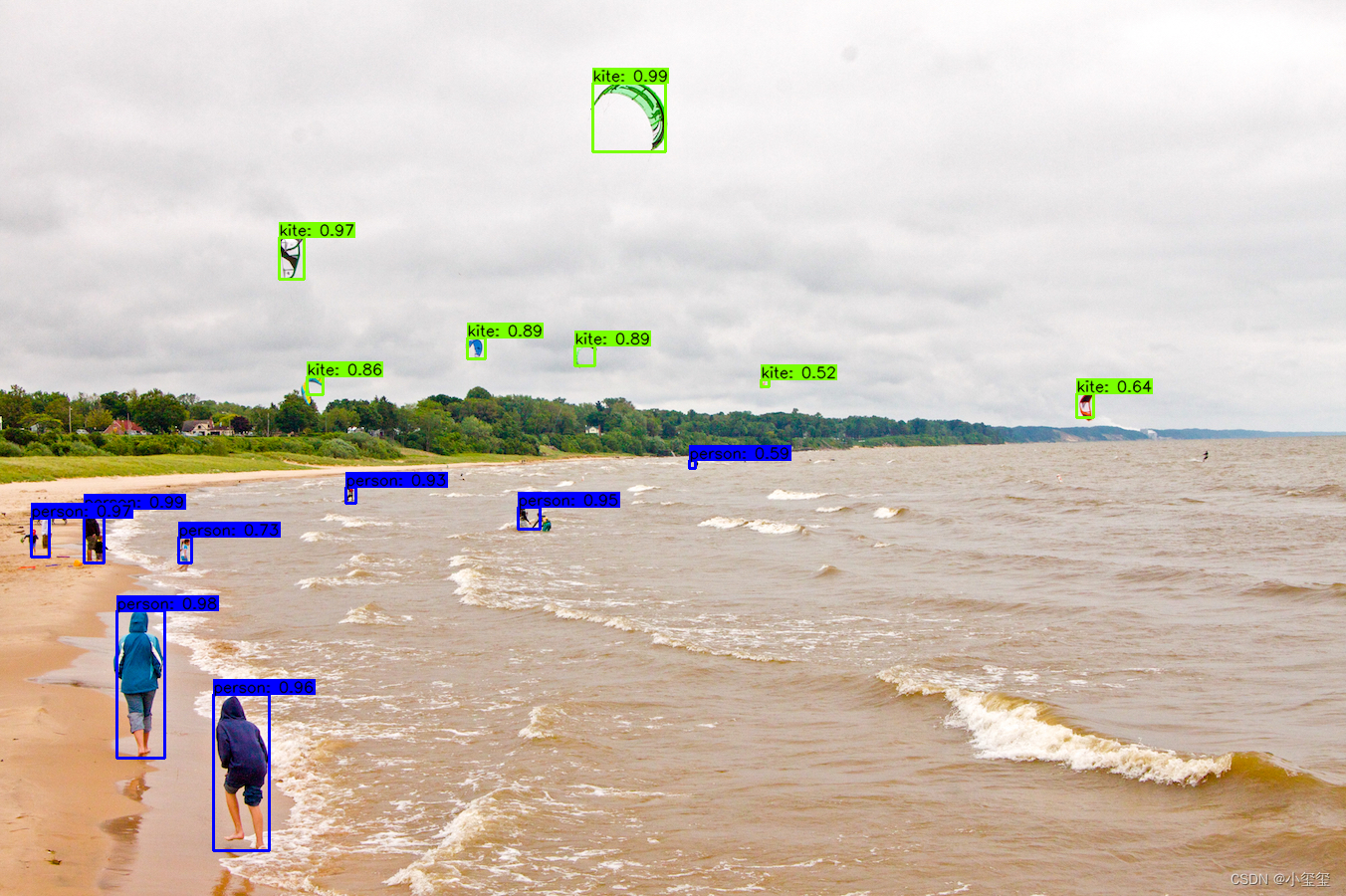
运行之后，我们可以得到检测结果。

2.1.5 上板运行

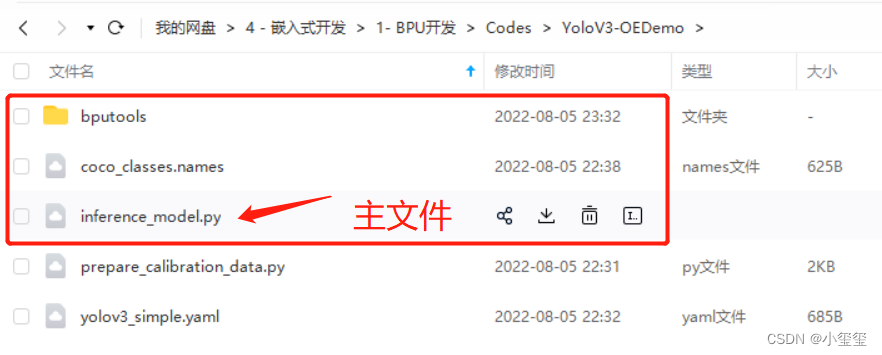
我们将下图所示的一些文件拖到旭日X3派开发板中，注意inference_model_bpu.py跟docker中是有微小的改动的。

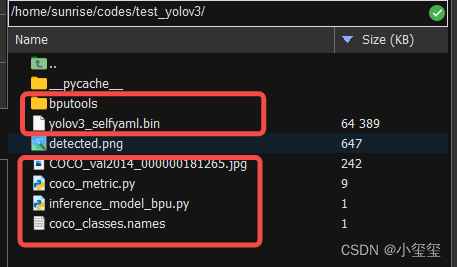
相关代码，放在百度云的test_yolov3文件夹下。

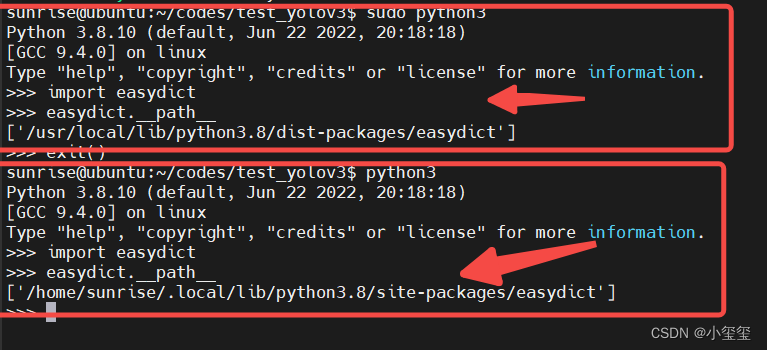
注意，在执行前要安装一些包sudo pip3 install EasyDict pycocotools，切记要加sudo，这样安装的路径不是用户目录，在运行BPU模型时候，也是必须要加sudo的。

inference_model_bpu.py的源码如下所示，与在docker中不同，nv12不需要再转为yuv444了，模型的运行也有一些差别。而后处理几乎没有变化。

import numpy as np
import cv2
import os
from hobot_dnn import pyeasy_dnn as dnn
from bputools.format_convert import imequalresize, bgr2nv12_opencv, nv122yuv444
from bputools.yolo_postproc import modelout2predbbox, recover_boxes, nms, draw_bboxs

def get_hw(pro):
    if pro.layout == "NCHW":
        return pro.shape[2], pro.shape[3]
    else:
        return pro.shape[1], pro.shape[2]

modelpath_prefix = ''

# img_path 图像完整路径
img_path = 'COCO_val2014_000000181265.jpg'
# model_path 量化模型完整路径
model_path = 'yolov3_selfyaml.bin'

# 1. 加载模型，获取所需输出HW
models = dnn.load(model_path)
model_h, model_w = get_hw(models[0].inputs[0].properties)

# 2 加载图像，根据前面模型，转换后的模型是以NV12作为输入的
# 但在OE验证的时候，需要将图像再由NV12转为YUV444
imgOri = cv2.imread(img_path)
img = imequalresize(imgOri, (model_w, model_h))
nv12 = bgr2nv12_opencv(img)

# 3 模型推理
t1 = cv2.getTickCount()
outputs = models[0].forward(nv12)
t2 = cv2.getTickCount()
outputs = (outputs[0].buffer, outputs[1].buffer, outputs[2].buffer)
print(outputs[0].shape, outputs[1].shape, outputs[2].shape)
# (1, 13, 13, 255) (1, 26, 26, 255) (1, 52, 52, 255)
print('time consumption {0} ms'.format((t2-t1)*1000/cv2.getTickFrequency()))

# 4 检测结果后处理
# 由output恢复416*416模式下的目标框
pred_bbox = modelout2predbbox(outputs)
# 将目标框恢复到原始分辨率
bboxes = recover_boxes(pred_bbox, (imgOri.shape[0], imgOri.shape[1]),
                       input_shape=(model_h, model_w), score_threshold=0.3)
# 对检测出的框进行非极大值抑制，抑制后得到的框就是最终检测框
nms_bboxes = nms(bboxes, 0.45)
print("detected item num: {0}".format(len(nms_bboxes)))

# 绘制检测框
draw_bboxs(imgOri, nms_bboxes)
cv2.imwrite('detected.png', imgOri)

• 1
• 2
• 3
• 4
• 5
• 6
• 7
• 8
• 9
• 10
• 11
• 12
• 13
• 14
• 15
• 16
• 17
• 18
• 19
• 20
• 21
• 22
• 23
• 24
• 25
• 26
• 27
• 28
• 29
• 30
• 31
• 32
• 33
• 34
• 35
• 36
• 37
• 38
• 39
• 40
• 41
• 42
• 43
• 44
• 45
• 46
• 47
• 48
• 49
• 50
• 51
• 52

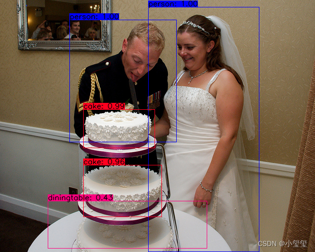
BPU上的检测结果如下图所示，推理耗时178ms，几乎赶上jetson TX2的性能了，开心。

2.1.6 小结

这里，对整个BPU部署流程我进行了一个梳理，如果按照官方教程，很简单，但我这里，想彻底完整地教会各位如何部署一个模型。

至少，校准数据、模型预处理、后处理、以及上板运行的代码都是我参考官方代码，一点点写出来的。我个人认为，这些代码能够让各位快速地理解这个过程的意义。

下面，以手部关键点检测网络，作为个测试，开始真正部署非官方的模型！！！！

2.2 手部关键点检测网络

手部关键点检测是做手势识别的一个关键过程，该代码基于Caffe，而且无自定义层，因此作为个引子，带领各位先初步使用BPU。

• 论文地址：Hand Keypoint Detection in Single Images using Multiview Bootstrapping
• 代码地址：github: learnopencv/HandPose/
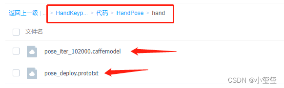
• Caffe模型：http://posefs1.perception.cs.cmu.edu/OpenPose/models/hand/pose_iter_102000.caffemodel
• 教程参考：《OpenCV手部关键点检测（手势识别）代码示例》

相关资料已经放在开头分享给各位的百度云里了（我把源码都放进去的目的是方便各位训练）

在转换BPU时，我们只需要对应的Prototxt和caffemodel文件，下面按照前面介绍的流程开始部署我们的模型。

2.2.1 模型准备

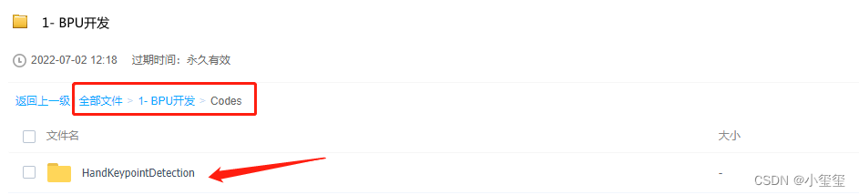
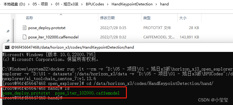
还记得在安装准备中，我们挂载了一个目录-v "D:\05 - 项目\01 - 旭日x3派\BPUCodes":/data/horizon_x3/codes吗，我们下载好代码后，按照如下方式放置相关文件，这时候我们就可以发现docker中也有这些文件啦。

2.2.2 验证模型

验证前，先将docker根目录切换到模型根目录下cd /data/horizon_x3/codes/HandKeypointDetection/hand/。

前面已经介绍了，模型验证需要利用hb_mapper checker后面跟一堆参数来对模型进行配置。下面带各位来配置这些参数：

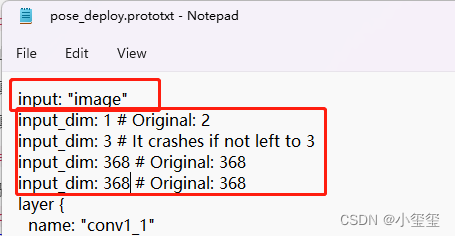
• --model-type：我们这些模型是Caffe，所以填caffe
• --march：旭日3派只能填bernoulli2
• --proto：填prototxt文件名，即pose_deploy.prototxt
• --model：填caffemodel文件名，即pose_iter_102000.caffemodel
• --input-shape：打开prototxt文件，查找input属性，可以发现模型只有一个输入，输入层的名称为image，输入图像的维度大小为1x3x368x368，那么这个参数设置就写为image 1x3x368x368。

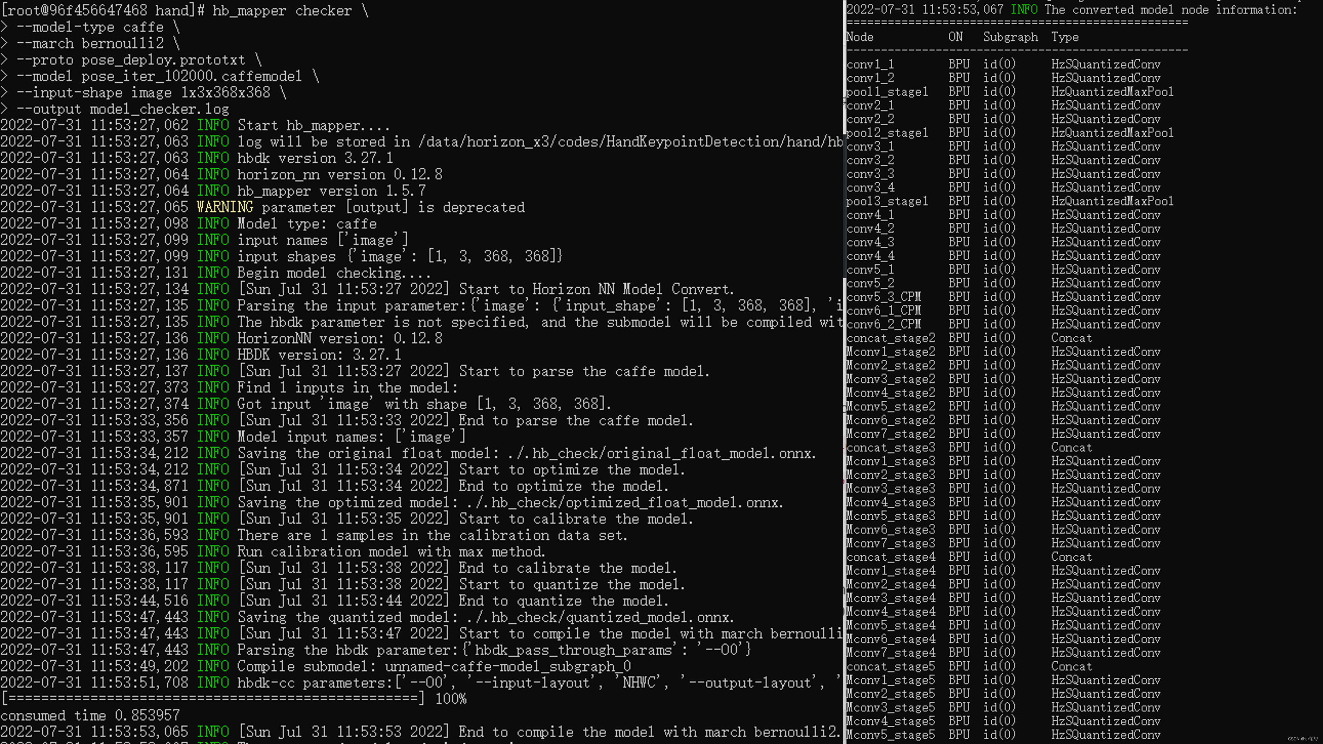
综上所述，在docker中需要输入如下指令来完成模型验证过程：

hb_mapper checker \
--model-type caffe \
--march bernoulli2 \
--proto pose_deploy.prototxt \
--model pose_iter_102000.caffemodel \
--input-shape image 1x3x368x368

• 1
• 2
• 3
• 4
• 5
• 6

输出结果如下所示，可以看到整个流程的转换状态以及每个节点是在BPU还是CPU上运行的。整个控制台的运行结果默认存在根目录的hb_mapper_checker.log中。

2.2.3 转换模型

与前面流程不同，这里我打算先配置yaml文件，再准备校准数据。

(i) 配置yaml文件

根据前文的思维导图，我们要进行配置。

• 模型参数组参数model_parameters配置：
  • output_model_file_prefix：给转换后的模型起个名，这里叫做'handkpdet'（hand keypoint detection）。
  • prototxt：caffe的prototxt，这里为'pose_deploy.prototxt'
  • caffe_model：caffe的模型文件，这里为'pose_iter_102000.caffemodel'
  • onnx_model：删掉。因为我们用的是Caffe。
• 输入信息组参数配置input_parameters：
  • input_type_train：原始浮点模型的输入数据格式，支持多种图像格式。我们这个模型，输入的是彩色图，考虑到opencv加载图像默认是BGR通道，因此这里设置为'bgr'。
  • input_layout_train：从前文的prototxt可以看出，数据输入排布为'NCHW'
  • input_type_rt：模型转换后，我们期望输入的图像格式。我们在训练模型和部署模型的时候，图像输入格式是可以变的，NV12是一些相机返回的原始数据格式，考虑到我们测试仍然基于本地图像，因此这里仍然设置为'bgr'。
  • norm_type：网络不可能拿原始图像数据作为输入的，一般都要进行一个归一化操作。这里用的模型对应的归一化代码为inpBlob = cv2.dnn.blobFromImage(frame, 1.0 / 255, (inWidth, inHeight), (0, 0, 0), swapRB=False, crop=False)，无减均值项，只有尺度项。因此，该属性设置为'data_scale'。
  • mean_value：删掉，因为网络没有均值项。
  • scale_value：尺度为1.0 / 255，因此设置为'0.0039'

最终，我们的yaml文件handpoint.yaml内容为：

model_parameters:
  prototxt: 'pose_deploy.prototxt'
  caffe_model: 'pose_iter_102000.caffemodel'
  output_model_file_prefix: 'handkpdet'
  march: 'bernoulli2'
input_parameters:
  input_type_train: 'bgr'
  input_layout_train: 'NCHW'
  input_type_rt: 'bgr'
  norm_type: 'data_scale'
  scale_value: '0.0039'
  input_layout_rt: 'NHWC'
calibration_parameters:
  cal_data_dir: './calibration_data'
  calibration_type: 'max'
  max_percentile: 0.9999
compiler_parameters:
  compile_mode: 'latency'
  optimize_level: 'O3'
  debug: False

• 1
• 2
• 3
• 4
• 5
• 6
• 7
• 8
• 9
• 10
• 11
• 12
• 13
• 14
• 15
• 16
• 17
• 18
• 19
• 20

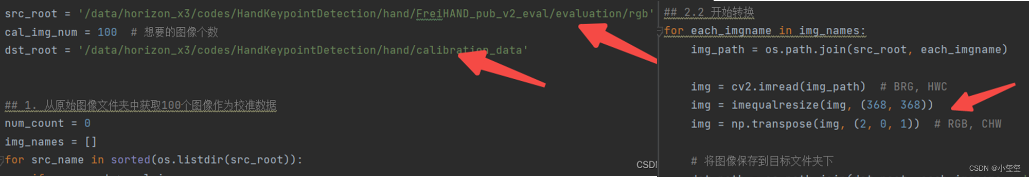
(ii) 准备校准数据

考虑到这个模型的输入只有一个，因此，准备校准数据部分的代码可以参考上一节的内容，需要修改的只有两个地方，原始数据地址，和颜色转换部分（取消了BGR转RGB的过程），数据集用的是FreiHAND_pub_v2_eval.zip，校准后的数据也放在了百度云里。

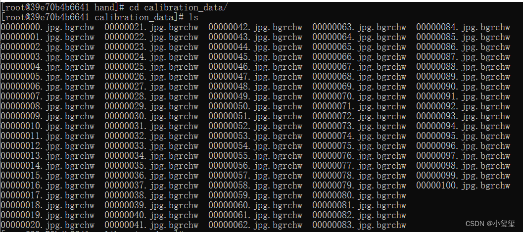
docker中，校准数据形式如下图所示，共计100张。

(iii) 开始转换

数据准备就绪，输入命令hb_mapper makertbin --config handpoint.yaml --model-type caffe开始转换我们的模型！
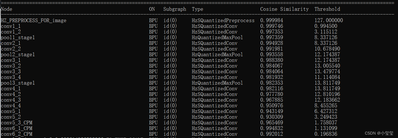
等待一段时间之后，模型转换成功，从结果可以看出来，模型的损失并不是很高！！感觉有戏，(☆▽☆)。

2.2.4 模型推理

由于该模型与前面的模型相似，都是以一张图像作为输入的，因此自己要补充的工作主要有两点：

• 完成图像预处理部分。前面的yaml文件指明了，量化后的模型是以BGR、NHWC格式作为输入的。因此，只需要调用resize成目标模型大小就行，opencv加载图像时候默认是HWC格式。
• 完成图像后处理部分。图像后处理一般与推理平台没有太大的关系，完整的流程都会有这个过程。

在docker中推理的完整代码如下所示。

import numpy as np
import cv2
import os
from horizon_tc_ui import HB_ONNXRuntime
import copy

# img_path 图像完整路径
img_path = '/data/horizon_x3/codes/HandKeypointDetection/hand/FreiHAND_pub_v2_eval/evaluation/rgb/00000253.jpg'
# model_path 量化模型完整路径
model_path = '/data/horizon_x3/codes/HandKeypointDetection/hand/model_output/handkpdet_quantized_model.onnx'

# 1. 加载模型，获取所需输出HW
sess = HB_ONNXRuntime(model_file=model_path)
sess.set_dim_param(0, 0, '?')
model_h, model_w = sess.get_hw()

# 2 加载图像，根据前面yaml，量化后的模型以BGR NHWC形式输入
imgOri = cv2.imread(img_path)
img = cv2.resize(imgOri, (model_w, model_h))

# 3 模型推理
input_name = sess.input_names[0]
output_name = sess.output_names
output = sess.run(output_name, {input_name: np.array([img])}, input_offset=128)
print(output_name)
print(output[0].shape)
# ['net_output']
# (1, 22, 46, 46)

# 4 检测结果后处理
# 绘制关键点
nPoints = 22
threshold = 0.1
POSE_PAIRS = [[0, 1], [1, 2], [2, 3], [3, 4], [0, 5], [5, 6], [6, 7], [7, 8], [0, 9], [9, 10], [10, 11], [11, 12],
              [0, 13], [13, 14], [14, 15], [15, 16], [0, 17], [17, 18], [18, 19], [19, 20]]

imgh, imgw = imgOri.shape[:2]
points = []
imgkp = copy.deepcopy(imgOri)
for i in range(nPoints):
    probMap = output[0][0, i, :, :]
    probMap = cv2.resize(probMap, (imgw, imgh))
    minVal, prob, minLoc, point = cv2.minMaxLoc(probMap)

    if prob > threshold:
        cv2.circle(imgkp, (int(point[0]), int(point[1])), 8, (0, 255, 255), thickness=-1, lineType=cv2.FILLED)
        cv2.putText(imgkp, "{}".format(i), (int(point[0]), int(point[1])), cv2.FONT_HERSHEY_SIMPLEX, 1, (0, 0, 255), 2,
                    lineType=cv2.LINE_AA)
        points.append((int(point[0]), int(point[1])))
    else:
        points.append(None)

# 绘制骨架
imgskeleton = copy.deepcopy(imgOri)
for pair in POSE_PAIRS:
    partA = pair[0]
    partB = pair[1]
    if points[partA] and points[partB]:
        cv2.line(imgskeleton, points[partA], points[partB], (0, 255, 255), 2)
        cv2.circle(imgskeleton, points[partA], 8, (0, 0, 255), thickness=-1, lineType=cv2.FILLED)
        cv2.circle(imgskeleton, points[partB], 8, (0, 0, 255), thickness=-1, lineType=cv2.FILLED)
# 保存关键点和骨架图
cv2.imwrite('handkeypoint.png', imgkp)
cv2.imwrite('imgskeleton.png', imgskeleton)

• 1
• 2
• 3
• 4
• 5
• 6
• 7
• 8
• 9
• 10
• 11
• 12
• 13
• 14
• 15
• 16
• 17
• 18
• 19
• 20
• 21
• 22
• 23
• 24
• 25
• 26
• 27
• 28
• 29
• 30
• 31
• 32
• 33
• 34
• 35
• 36
• 37
• 38
• 39
• 40
• 41
• 42
• 43
• 44
• 45
• 46
• 47
• 48
• 49
• 50
• 51
• 52
• 53
• 54
• 55
• 56
• 57
• 58
• 59
• 60
• 61
• 62
• 63
• 64

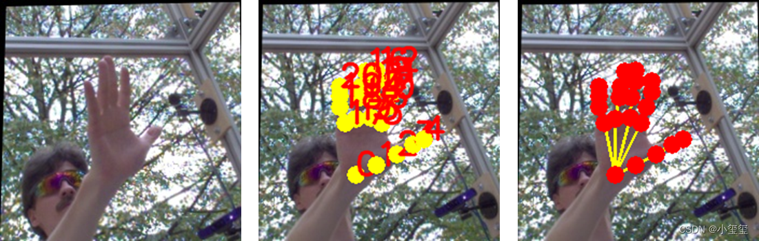
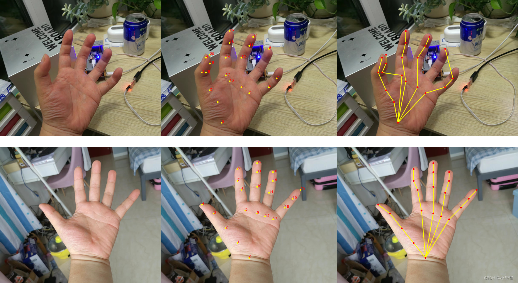
最终结果图如下图所示，感觉还蛮不错哦

2.2.5 上板运行

在开发板运行的程序与上述推理代码差异不大，注意好模型的输入数据格式即可，这里要注意，输出的outputs与docker中有差异，要做output = (outputs[0].buffer,)转换，这样可以直接兼容后面的后处理部分，进而生成结果图。

整个板端运行代码放在百度云中的test_handpose文件夹

import numpy as np
import cv2
import os
from hobot_dnn import pyeasy_dnn as dnn
import copy

def get_hw(pro):
    if pro.layout == "NCHW":
        return pro.shape[2], pro.shape[3]
    else:
        return pro.shape[1], pro.shape[2]

# img_path 图像完整路径
img_path = '20220806023323.jpg'
# model_path 量化模型完整路径
model_path = 'handkpdet.bin'

# 1. 加载模型，获取所需输出HW
models = dnn.load(model_path)
model_h, model_w = get_hw(models[0].inputs[0].properties)

# 2 加载图像，根据前面yaml，量化后的模型以BGR NHWC形式输入
imgOri = cv2.imread(img_path)
img = cv2.resize(imgOri, (model_w, model_h))

# 3 模型推理
t1 = cv2.getTickCount()
outputs = models[0].forward(img)
t2 = cv2.getTickCount()
output = (outputs[0].buffer,)
print(outputs[0].buffer.shape)
# (1, 22, 46, 46)
print('time consumption {0} ms'.format((t2-t1)*1000/cv2.getTickFrequency()))


# 4 检测结果后处理
# 绘制关键点
nPoints = 22
threshold = 0.1
POSE_PAIRS = [[0, 1], [1, 2], [2, 3], [3, 4], [0, 5], [5, 6], [6, 7], [7, 8], [0, 9], [9, 10], [10, 11], [11, 12],
              [0, 13], [13, 14], [14, 15], [15, 16], [0, 17], [17, 18], [18, 19], [19, 20]]

imgh, imgw = imgOri.shape[:2]
points = []
imgkp = copy.deepcopy(imgOri)
for i in range(nPoints):
    probMap = output[0][0, i, :, :]
    probMap = cv2.resize(probMap, (imgw, imgh))
    minVal, prob, minLoc, point = cv2.minMaxLoc(probMap)

    if prob > threshold:
        cv2.circle(imgkp, (int(point[0]), int(point[1])), 8, (0, 255, 255), thickness=-1, lineType=cv2.FILLED)
        cv2.putText(imgkp, "{}".format(i), (int(point[0]), int(point[1])), cv2.FONT_HERSHEY_SIMPLEX, 1, (0, 0, 255), 2,
                    lineType=cv2.LINE_AA)
        points.append((int(point[0]), int(point[1])))
    else:
        points.append(None)

# 绘制骨架
imgskeleton = copy.deepcopy(imgOri)
for pair in POSE_PAIRS:
    partA = pair[0]
    partB = pair[1]
    if points[partA] and points[partB]:
        cv2.line(imgskeleton, points[partA], points[partB], (0, 255, 255), 2)
        cv2.circle(imgskeleton, points[partA], 8, (0, 0, 255), thickness=-1, lineType=cv2.FILLED)
        cv2.circle(imgskeleton, points[partB], 8, (0, 0, 255), thickness=-1, lineType=cv2.FILLED)
# 保存关键点和骨架图
cv2.imwrite('handkeypoint.png', imgkp)
cv2.imwrite('imgskeleton.png', imgskeleton)

• 1
• 2
• 3
• 4
• 5
• 6
• 7
• 8
• 9
• 10
• 11
• 12
• 13
• 14
• 15
• 16
• 17
• 18
• 19
• 20
• 21
• 22
• 23
• 24
• 25
• 26
• 27
• 28
• 29
• 30
• 31
• 32
• 33
• 34
• 35
• 36
• 37
• 38
• 39
• 40
• 41
• 42
• 43
• 44
• 45
• 46
• 47
• 48
• 49
• 50
• 51
• 52
• 53
• 54
• 55
• 56
• 57
• 58
• 59
• 60
• 61
• 62
• 63
• 64
• 65
• 66
• 67
• 68
• 69
• 70

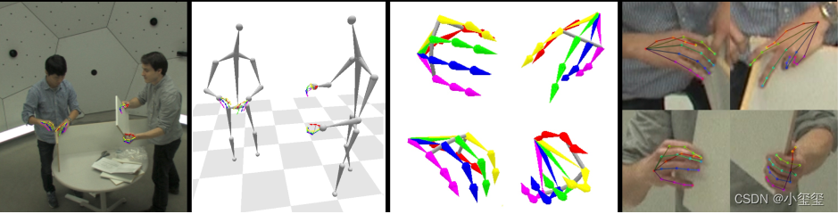
我自己拍了两张图进行测试，第一排是晚上拍的，手指头有点串味哈哈，整体检测耗时在480ms左右，网络深度没有yolo高，也许是横向的特征比较多。

2.2.6 小结

BPU的学习，最难的就是第一步，成功捋清楚yolo的部署方式后，这个手部关键点检测按照这个教程就不到1个小时就搞定了。

三 总结

花费了将近两个月，总共耗时60多个小时，我终于把BPU的基础部分搞的差不多明白了，昨晚是一鼓作气搞到快凌晨3点，早上起来后赶紧把代码流程整理下，兴奋地都没睡好。

这是我耗时最多，周期最长的一个博客了，所以关于其中的优缺点，我要多多说一说。先列优点：

• 整个工具链很完整，demo很全，能覆盖基于CNN的各种情况的网络模型，你甚至可以把网络某个层的输出拿出来，以数据类型为feature作为下一个模型的输入。
• 5TOPS的BPU速度比我想象的要快很多，而且网络推理过程只用了1个BPU核，如果开2个核计算的话，时间还能优化30%左右。
• 官方的技术支持很热情（感觉最后都被我问烦了，逃）

关于缺点，也是很明显，最致命的就是官方文档无法有效引导新手上手BPU，但我希望这个博客能够缓解这个问题，因为只要成功走了一次，之后的工作就会轻松很多。

• yaml的配置不循序渐进。总共30多个参数，但是不是所有的网络都要一个个检查遍这个参数，对于新手来说，我们只需要快速部署，其他好多参数是高级功能，可以后续根据需求去学习的。
• 增加技术支持人员。我对一个东西喜欢研究的很细，逮着一个人疯狂问，估计都烦了（反正我会了，这个不改进也行ε=ε=ε=┏(゜ロ゜;)┛）
• demo代码没有必要写的那么专业，那么智能。有些转换函数，比如demo中提供了多种格式变换函数，比如nv12等，可以直接放进python的site-packages里面。
• 还有一个小小的建议，冷门包（比如EasyDict pycocotools等）安装几乎都要板端编译，要等很久，希望官方能够提供个镜像。这些冷门包可以由官方编译或者用户编译好上传。

BPU要降低学习成本，我个人认为非常重要。（我读书时候都不爱看书听课，还能专心下来看这么多文档？→_→）