首页 最新 热门 推荐

登录

• 首页
• 最新
• 热门
• 推荐

21天学通C++读书笔记（二十五：理解智能指针）

• 23-11-18 01:40
• 3376
• 11397

blog.csdn.net

1. 什么是智能指针

• C++智能指针是包含重载运算符的类，其行为像常规指针，但智能指针能够及时、妥善地销毁动态分配的数据，并实现了明确的对象生命周期，因此更有价值

1.1 常规（原始）指针存在的问题

• 与其他现代编程语言不同，C++在内存分配、释放和管理方面向程序员提供了全面的灵活性
• 但同时，也制造了与内存相关的问题，如动态分配的对象没有正确地释放时将导致内存泄露

SomeClass* ptrData = anObject.GetData();
ptrData->DoSomething();
1
2

• 在上述代码中，没有显而易见的方法获悉 ptrData 指向的内存

• 是否是从堆中分配的，因此最终需要释放
• 是否由调用者负责释放
• 对象的析构函数是否会自动销毁该对象

1.2 智能指针有何帮助

• 当需要管理堆（自由存储区）中数据时，可在程序中使用智能指针，以更智能的方式分配和管理内存

smart_pointer<SomeClass> spData = anObject.GetData();
spData->Display();
(*spData).Display();
// 智能指针的行为类似常规指针，但通过重载的运算符和析构函数可确保动态分配的数据能够及时地销毁
1
2
3
4

2. 智能指针是如何实现的

• 智能指针类重载了解除引用运算符（*）和成员选择运算符（->），可以像使用常规指针那样使用它们
• 另外，为了能够在堆中管理各种类型，几乎所有的智能指针类都是模板类，包含其功能的泛型实现。由于模板是通用的，可以根据要管理的对象类型进行具体化

template<typename T>
class smart_pointer {
private:
    T* rawPtr;
public:
    // 构造函数接受一个指针，并将其保存到该智能指针类内部的一个指针对象中
    smart_pointer (T* pData) : rawPtr (pData) {}
    // 析构函数释放该指针，从而实现了自动内存释放
    ~smart_pointer () {delete rawPtr;};
    
    // copy constructor
    smart_pointer (const smart_pointer & anotherSP);
    // copy assignment operator
    smart_pointer& operator= (const smart_pointer& anotherSP);    
    
    T& operator* () const {   // 重载了 * 运算符
        return *(rawPtr);
    }
    T* operator-> () const {  // 重载了 -> 运算符
        return rawPtr;
    }
};

int main() {
	return 0;
}
1
2
3
4
5
6
7
8
9
10
11
12
13
14
15
16
17
18
19
20
21
22
23
24
25
26

使智能指针真正“智能”的是复制构造函数、赋值运算符和析构函数的实现，它们决定了智能指针对象被传递给函数、赋值或离开作用域（即像其他类对象一样被销毁）时的行为

3. 智能指针类型

• 智能指针决定在复制和赋值时如何处理内存资源
• 智能指针的分类实际上就是内存资源管理策略的分类，可分为如下几类
  • 深复制
  • 写时复制（Copy on Write，COW）
  • 引用计数
  • 引用链接
  • 破坏性复制

3.1 深复制

• 在实现深复制的智能指针中，每个智能指针实例都保存一个它管理的对象的完整副本
• 每当智能指针被复制时，将复制它指向的对象（因此称为深复制）
• 每当智能指针离开作用域时，将（通过析构函数）释放它指向的内存

虽然基于深复制的智能指针看起来并不比按值传递对象优越，但在处理多态对象时，其优点将显现出来

// 使用基于深复制的智能指针将多态对象作为基类对象进行传递
template<typename T>
class deepcopy_smart_ptr {
private:
    T* object;
public:
    //... other functions
    
    // 深复制指针的复制构造函数
    // 使得能够通过Clone()函数对多态对象进行深复制——类必须实现函数Clone()
    deepcopy_smart_ptr (const deepcopy_smart_ptr& source) {
        // Clone() is virtual: ensures deep copy of Derived class object
        object = source->Clone();
    }
    
    // 复制赋值运算符
    deepcopy_smart_ptr& operator= (const deepcopy_smart_ptr& source) {
        if (object) {
            delete object;
        }
        object = source->Clone();
    }
};

int main() {
    deepcopy_smart_ptr<Carp> freshWaterFish(new Carp);
    MakeFishSwim (freshWaterFish);

    return 0;
}
1
2
3
4
5
6
7
8
9
10
11
12
13
14
15
16
17
18
19
20
21
22
23
24
25
26
27
28
29
30

基于深复制的机制的不足之处在于性能，这可能不使用智能指针，而将指向基类的指针（常规指针Fish*）传递给函数

3.2 写时复制机制

• 写时复制机制（Copy on Write，COW）试图对深复制智能指针的性能进行优化，它共享指针，直到首次写入对象
• 首次调用非 const 函数时，COW 指针通常为该非 const 函数操作的对象创建一个副本，而其他指针实例仍共享源对象

3.3 引用计数智能指针

• 引用计数是一种记录对象的用户数量的机制，当计数降低到零后，便将对象释放
• 引用计数提供了一种优良的机制，使得可共享对象而无法对其进行复制

这种智能指针被复制时，需要将对象的引用计数加1，至少有两种常用的方法来跟踪计数

• 在对象中维护引用计数(称为入侵式引用计数，因为需要修改对象以维护和递增引用计数，并将其提供给管理对象的智能指针，COM 采取的就是这种方法)
• 引用计数由共享对象中的指针类维护 { 智能指针类将计数保存在自由存储区（如动态分配的整型），复制时复制构造函数将这个值加1 }

• 使用引用计数机制，程序员只应通过智能指针来处理对象。在使用智能指针管理对象的同时让原始指针指向它是一种糟糕的做法，因为智能指针将在它维护的引用计数减为零时释放对象，而原始指针将继续指向已不属于当前应用程序的内存
• 引用计数还有一个独特的问题
  • 如果两个对象分别存储指向对方的指针，这两个对象将永远不会被释放，因为它们的生命周期依赖性导致其引用计数最少为1

3.4 引用链接智能指针

• 引用链接智能指针不主动维护对象的引用计数，而只需知道计数什么时候变为零，以便能够释放对象
• 之所以称为引用链接，是因为其实现是基于双向链表的，通过复制智能指针来创建新智能指针时，新指针将被插入到链表中；当智能指针离开作用域进而被销毁时，析构函数将把它从链表中删除
• 与引用计数的指针一样，引用链接指针也存在生命周期依赖性导致的问题

3.5 破坏性复制

• 破坏性复制是这样一种机制，即在智能指针被复制时，将对象的所有权转交给目标指针并重置原来的指针
• 虽然破坏性复制机制使用起来并不直观，但它有一个优点：即可确保任何时刻只有一个活动指针指向对象。因此，它非常适合从函数返回指针以及需要利用其“破坏性”的情形
• std::auto_ptr 是最流行的破坏性复制指针，被传递给函数或复制给另一个指针后，这种智能指针就没有用了（该智能指针类的复制构造函数和赋值运算符不能接受const 引用）

C++11 摒弃了 std::auto_ptr，应使用 std::unque_ptr，这种指针不能按值传递，而只能按引用传递，因为其复制构造函数和复制赋值运算符都是私有的

template<typename T>
class destructivecopy_ptr {
private:
    T* object;
public:
    destructivecopy_ptr(T* input):object(input) {}
    ~destructivecopy_ptr() { delete object; }
    
    // 这些函数实际上在源指针被复制后失效，即复制构造函数在复制后将源指针设
    // 置为NULL，这就是“破坏性复制”的由来
    destructivecopy_ptr(destructivecopy_ptr& source) {
        // Take ownership on copy
        object = source.object;
        // destroy source
        source.object = 0;
    }
    // 复制赋值运算符亦如此
    destructivecopy_ptr& operator= (destructivecopy_ptr& source) {
        if (object != source.object) {
            delete object;
            object = source.object;
            source.object = 0;
        }
    }
};

int main() {
    destructivecopy_ptr<int> num (new int);
    destructivecopy_ptr<int> copy = num;
    
    // num is now invalid
    return 0;
}
1
2
3
4
5
6
7
8
9
10
11
12
13
14
15
16
17
18
19
20
21
22
23
24
25
26
27
28
29
30
31
32
33

3.6 使用std::unique_ptr

• std::unique_ptr 是 C++11 新增的，与 auto_ptr 稍有不同，因为它不允许复制和赋值
• 其复制构造函数和赋值运算符被声明为私有的，故不能复制它，即不能将其按值传递给函数，也不能将其赋给其他指针

#include 
#include 
using namespace std;

class Fish {
public:
    Fish() {cout << "Fish: Constructed!" << endl;}
    ~Fish() {cout << "Fish: Destructed!" << endl;}
    
    void Swim() const {cout << "Fish swims in water" << endl;}
};

void MakeFishSwim(const unique_ptr<Fish>& inFish) {
    inFish->Swim();
}

int main() {
    unique_ptr<Fish> smartFish (new Fish);
    
    smartFish->Swim();
    MakeFishSwim(smartFish); // OK, as MakeFishSwim accepts reference
    
    unique_ptr<Fish> copySmartFish;
    // copySmartFish = smartFish; // error: operator= is private
    
    unique_ptr<Fish> sameFish (std::move(smartFish)); 
    // smartFish is empty henceforth
    
    return 0;
}
1
2
3
4
5
6
7
8
9
10
11
12
13
14
15
16
17
18
19
20
21
22
23
24
25
26
27
28
29
30

Fish: Constructed!
Fish swims in water
Fish swims in water
Fish: Destructed!
1
2
3
4

编写多线程的应用程序时，可考虑使用 std::shared_ptr 和 std::weak_ptr，它们可帮助实现线程安全和引用计数对象共享

Q&A

• string 类在自由存储区中动态地管理字符数组，它也是智能指针吗？
  • 不是。string 类通常没有实现运算符*和−>，因此不属于智能指针。

id="article_content" class="article_content clearfix"> id="content_views" class="markdown_views prism-atom-one-dark">

Question 1: What are the conceptual connections between state space models and attention? Can we combine them?
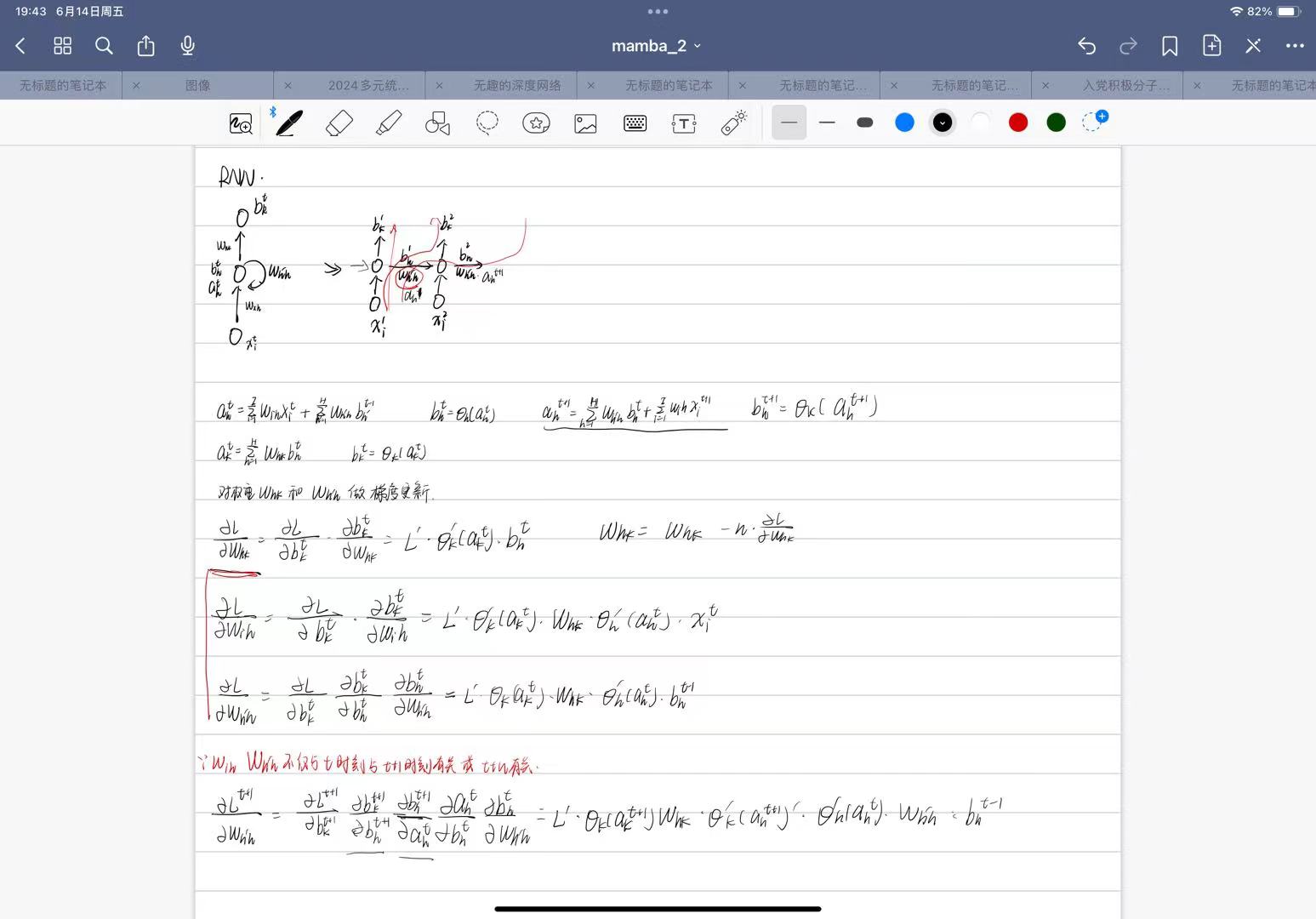
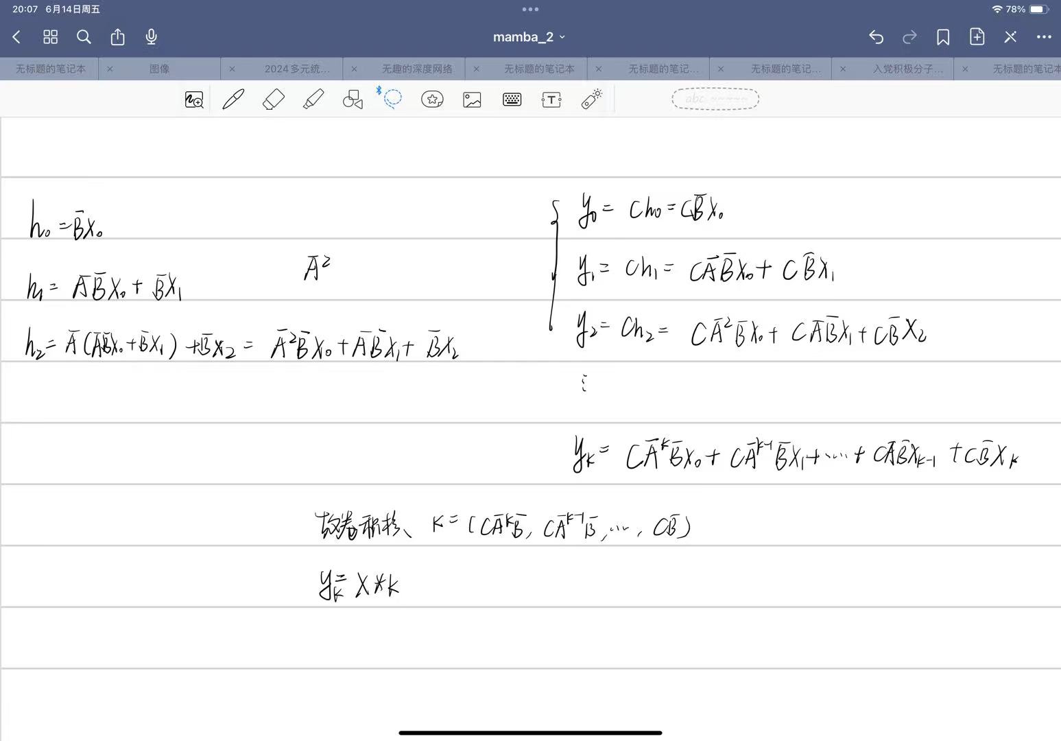
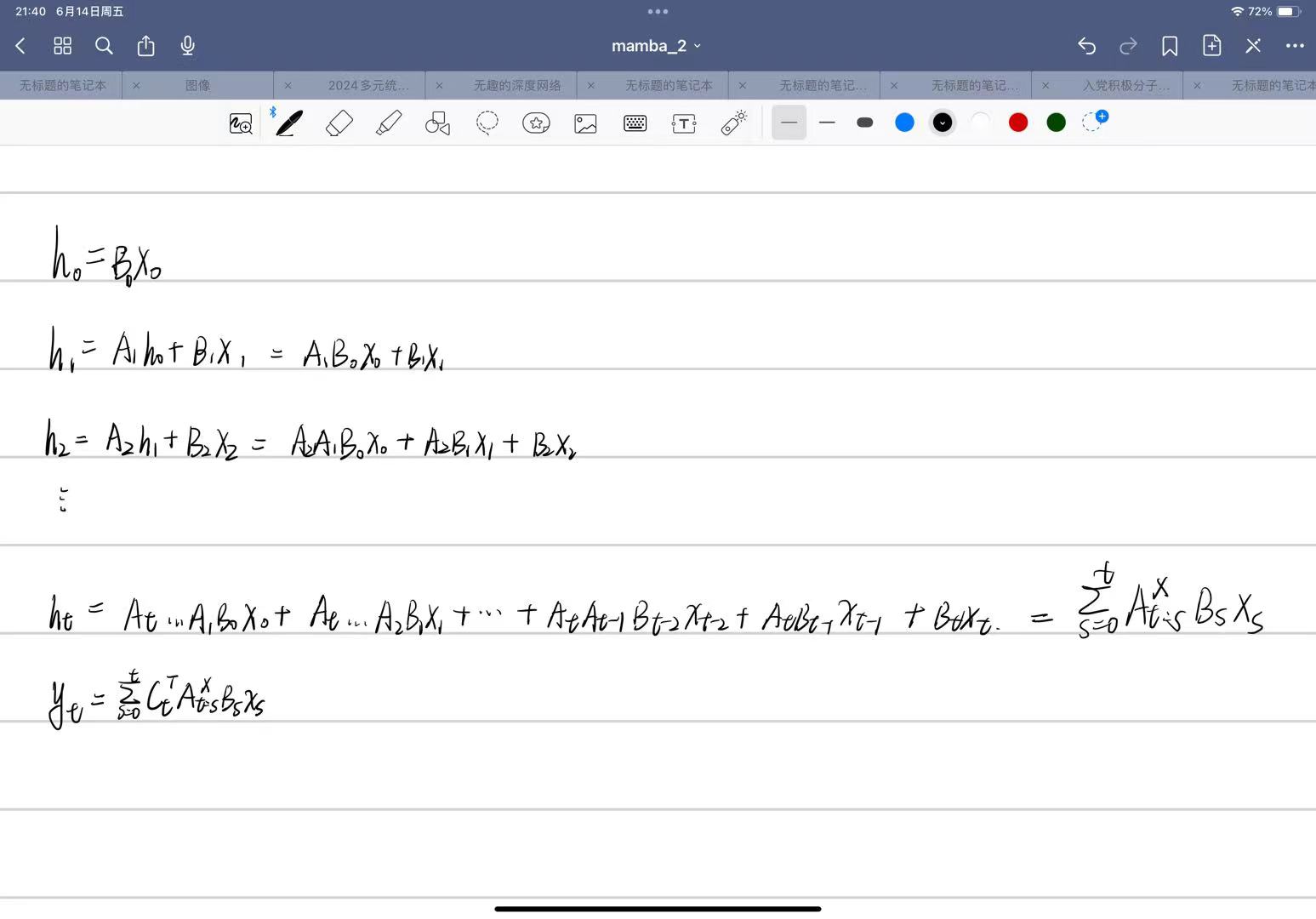
从概念的角度来看，发现 SSM 如此迷人的原因之一是给人的感觉就像_基础_一样。其中一个例子就是它们与许多主要的序列模型范式有着密切的联系。正在结构化 SSM 方面的工作中所阐述的那样，它们似乎抓住了连续、卷积和循环序列模型的本质——所有这些都包含在一个简单而优雅的模型中。（底下会介绍）
当然，除了这些之外，还有另一个主要的序列模型范式：无处不在的注意力机制的变体。SSM 总是让人感觉与注意力有些脱节，我们尝试了一段时间来更好地理解它们之间的关系
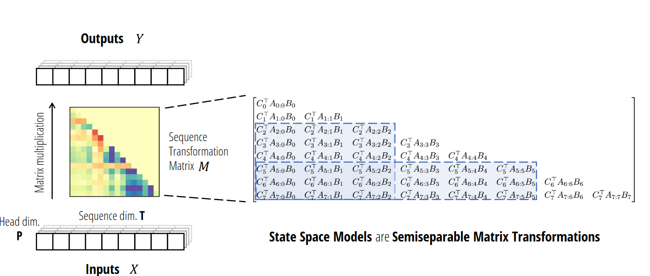
_Question 2: _Can we speed up the training of Mamba models by recasting them as matrix multiplications?
从计算的角度来看，尽管 Mamba 为提高速度付出了很多努力（特别是其硬件感知选择性扫描实现），但它的硬件效率仍然远低于注意力机制。缺少的一点是，现代加速器（如 GPU 和 TPU）_高度_专门用于矩阵乘法。虽然这对于推理来说不是问题，因为推理的瓶颈在于不同的考虑因素，但这在训练期间可能是一个大问题。

环境配置

安装依赖

conda create -n mamba python=3.10
conda activate mamba
conda install cudatoolkit==11.8 -c nvidia
pip install torch==2.3.1 torchvision==0.18.1 torchaudio==2.3.1 --index-url https://pypi.tuna.tsinghua.edu.cn/simple
pip install triton==2.3.1
pip install transformers==4.43.3
pip install ninja --index-url https://pypi.tuna.tsinghua.edu.cn/simple
 class="hljs-button signin active" data-title="登录复制" data-report-click="{"spm":"1001.2101.3001.4334"}">

• 1
• 2
• 3
• 4
• 5
• 6
• 7

安装CUDA_NVCC

conda install -c "nvidia/label/cuda-11.8.0" cuda-nvcc
 class="hljs-button signin active" data-title="登录复制" data-report-click="{"spm":"1001.2101.3001.4334"}">

• 1

找到CUDA11.8的libcudart.so

find ~/miniconda3/ -name libcudart.so
 class="hljs-button signin active" data-title="登录复制" data-report-click="{"spm":"1001.2101.3001.4334"}">

• 1

你会得到一个…/miniconda3/pkgs/cudatoolkit-11.8.0-h6a678d5_0/lib/libcudart.so的路径
将其写入到bashrc中作为CUDA11.8的路径

echo 'export LD_LIBRARY_PATH=/miniconda3/pkgs/cudatoolkit-11.8.0-h6a678d5_0/lib:$LD_LIBRARY_PATH' >> ~/.bashrc
source ~/.bashrc
 class="hljs-button signin active" data-title="登录复制" data-report-click="{"spm":"1001.2101.3001.4334"}">

• 1
• 2

之后你就可以愉快的测试你的代码了

# mamba1
import torch
from mamba_ssm import Mamba

batch, length, dim = 2, 64, 16
x = torch.randn(batch, length, dim).to("cuda")
model = Mamba(
    # This module uses roughly 3 * expand * d_model^2 parameters
    d_model=dim, # Model dimension d_model
    d_state=16,  # SSM state expansion factor
    d_conv=4,    # Local convolution width
    expand=2,    # Block expansion factor
).to("cuda")
y = model(x)
print(y.shape)

# mamba2
from mamba_ssm import Mamba2
model = Mamba2(
    # This module uses roughly 3 * expand * d_model^2 parameters
    d_model=dim, # Model dimension d_model
    d_state=64,  # SSM state expansion factor, typically 64 or 128
    d_conv=4,    # Local convolution width
    expand=2,    # Block expansion factor
).to("cuda")
y = model(x)
assert y.shape == x.shape
 class="hljs-button signin active" data-title="登录复制" data-report-click="{"spm":"1001.2101.3001.4334"}">

class="hide-preCode-box">

• 1
• 2
• 3
• 4
• 5
• 6
• 7
• 8
• 9
• 10
• 11
• 12
• 13
• 14
• 15
• 16
• 17
• 18
• 19
• 20
• 21
• 22
• 23
• 24
• 25
• 26
• 27

The Model

The SSD Model

Mamba-2 论文的重点是结构化状态空间对偶性（SSD），它指的是几件事：

1. SSD 模型是指可以纳入深度神经网络的特定独立层，如注意力机制或 SSM
2. SSD 框架是推理此模型（以及更多理论联系）的通用框架
3. SSD 算法是一种比以前的 SSM 更有效地计算 SSD 层的算法

线性时不变系统-线性（SSMs）模型

解释线性时不变系统（Linear Time-Invariant System，简称LTI系统）：是控制理论和信号处理中的一个基本概念。它描述了一个系统，其输出与输入之间的关系是线性的，并且不随时间改变。
h t = A h t − 1 + B x t y t = C ⊤ h t class="MathJax_Display">ht=Aht−1+Bxtyt=C⊤ht" role="presentation">ht=Aht−1+Bxtyt=C⊤ht$$\begin{array}{rl}& h_t=A{h}_{t-1}+B{x}_t\\ & y_t=C^{\mathrm{\top }}{h}_t\end{array}$$ ​ht​=Aht−1​+Bxt​yt​=C⊤ht​​ （0） h t = A t h t − 1 + B t x t y t = C t ⊤ h t class="MathJax_Display">ht=Atht−1+Btxtyt=Ct⊤ht" role="presentation">htyt=Atht−1+Btxt=C⊤tht$$\begin{array}{rl}{h}_t& =A_t{h}_{t-1}+B_t{x}_t\\ y_t& =C_t^{\mathrm{\top }}{h}_t\end{array}$$ ht​yt​​=At​ht−1​+Bt​xt​=Ct⊤​ht​​ （1）
A selective state space model 是允许（A，B，C）随着时间变化而变化的，通常将其看作带有形状的张量，其中$A\in {\mathbb{R}}^{(\mathrm{T},\mathrm{N},\mathrm{N})},B\in {\mathbb{R}}^{(\mathrm{T},\mathrm{N})},\mathrm{and}C\in {\mathbb{R}}^{(\mathrm{T},\mathrm{N})}$。结构化 SSM 需要_A_具有可有效计算的结构，例如最常用的对角线结构，在这种情况下_A_有形状（T ，N ）其中只有对角线元素矩阵被存储。

RNN模型

h t = f ( W x h x t + W h h h t − 1 ) y t = g ( W h y h t ) , class="MathJax_Display">ht=f(Wxhxt+Whhht−1)yt=g(Whyht)," role="presentation">ht=f(Wxhxt+Whhht−1)yt=g(Whyht),$$\begin{array}{rl}& {\mathit{h}}_t=f({\mathit{W}}_{xh}{\mathit{x}}_t+{\mathit{W}}_{hh}{\mathit{h}}_{t-1})\\ & {\mathit{y}}_t=g({\mathit{W}}_{hy}{\mathit{h}}_t),\end{array}$$ ​ht​=f(Wxh​xt​+Whh​ht−1​)yt​=g(Why​ht​),​
思考：SSM模型作为状态空间模型与RNN结构想类似为什么，可以避免梯度消失。（ssm线性）

CNN模型

当SSM的动力学特性一样，在时间上是常数时，该模型被称为线性时不变( LTI ) 。在这种情况下，它们等价于卷积。

SSD：标量结构化SSM

原始的Mamba（或者更准确地说是其核心的“S6”层）正是具有对角结构的选择性SSM。
Mamba-2 的 SSD 层只做了一个小修改：它限制了对角线A甚至进一步变成标量乘以恒等结构；换句话说A必须全部为相同值。在这种情况下A可以用形状 (T)来表示还可以识别只是一个标量（所以有时会表示它）。
方程（1）仅针对单维输入进行定义，仅针对单维输入进行定义$x\in {\mathbb{R}}^{\mathrm{T}}$。 如果$X\in {\mathbb{R}}^{(\mathrm{T},\mathrm{P})}$有P个不同的通道，作者使用相同的动态（即相同的 SSM) 独立地针对每个通道。这可以解释为SSM 模型的_单个头。_在这里，作者认为$\mathbf{X}$这是一个形状张量，$(\mathrm{T},\mathrm{P})$其中$\mathrm{T}$是序列（时间）维度，$\mathrm{P}$是“头部维度”。
多个头可以完全独立地构建；在这篇文章的其余部分中，作者假设使用的是一个头。请注意，这些头部与多头注意力模型中的头部的工作原理完全相似，在Mamba-2中，作者也选择了与现代变形金刚相似的尺寸，例如$\mathrm{P}=64$或$\mathrm{P}=128$。（为了扩展到更大的模型宽度，保持这个固定，并增加独立头的数量。）
$Y^{(\mathrm{T},\mathrm{P})}=\mathrm{SSM}(A^{(\mathrm{T},\dots )},B^{(\mathrm{T},\mathrm{N})},C^{(\mathrm{T},\mathrm{N})})(X^{(\mathrm{T},\mathrm{P})})$ （2）
一些变化包括:

1. 结构_A_，这会影响其参数形状：
   • ⋯ = ( N , N ) class="MathJax_Display">⋯=(N,N)" role="presentation">⋯=(N,N)$$\begin{array}{ccc}\cdots & =& (\mathrm{N},\mathrm{N})\end{array}$$ ⋯​=​(N,N)​对于一般（非结构化）SSM
   • ⋯ = ( N ) class="MathJax_Display">⋯=(N)" role="presentation">⋯=(N)$$\begin{array}{ccc}\cdots & =& (\mathrm{N})\end{array}$$ ⋯​=​(N)​对于对角线 SSM（或其他结构，例如对角线加低秩）
   • ⋯ = ( ) class="MathJax_Display">⋯=()" role="presentation">⋯=()$$\begin{array}{ccc}\cdots & =& ()\end{array}$$ ⋯​=​()​对于标量 SSM（即 SSD）
2. The state dimension N(i.e. d_state)
3. The head dimension P(i.e. d_head)

SSD层的双重注意样形式是
$M=L\circ C{B}^{\top }\in {\mathbb{R}}^{(\mathrm{T},\mathrm{T})}$

State Space Models are Structured Matrices

状态空间模型与称为半可分离矩阵的结构化矩阵族之间的等价性

Matrix Transformations

其思想是许多序列模型，即序列变换$X\in {\mathbb{R}}^{(\mathrm{T},\mathrm{P})}\mapsto Y\in {\mathbb{R}}^{(\mathrm{T},\mathrm{P})}$，可以写成单一矩阵乘法的形式$Y=M(X)\cdot X$，其中是一个本身可以依赖的矩阵$X$。我们称之为矩阵序列变换，或简称矩阵变换。在文献中，序列变换也被称为“序列混合器”或“标记混合器”，而矩阵序列变换则被称为“矩阵混合器”。其中有许多这些例子，它们可以通过矩阵的结构来区分。事实上的例子是自我注意本身，$M=\mathrm{softmax}(Q{K}^{\top })$其中是注意力矩阵。其他的例子包括MLP-Mixer，FNet，和Monarch Mixer。
为什么我们要关心这些类型的模型呢？
将序列模型作为矩阵转换来编写，为理解模型的结构和特征提供了一个强大的工具
虽然一般的非线性RNNs，如LSTMs不能写成矩阵形式，但状态空间模型可以！事实上，仅仅通过展开SSM递归的定义，就很容易看到这一点。其结果是，SSM (2) 可以写成一个矩阵变换
$Y=\mathsf{SSM}(A,B,C)(X)=MX$
h t = A t … A 1 B 0 x 0 + A t … A 2 B 1 x 1 + ⋯ + A t A t − 1 B t − 2 x t − 2 + A t B t − 1 x t − 1 + B t x t = ∑ s = 0 t A t : s × B s x s . class="MathJax_Display">ht=At…A1B0x0+At…A2B1x1+⋯+AtAt−1Bt−2xt−2+AtBt−1xt−1+Btxt=∑s=0tAt:s×Bsxs." role="presentation">ht=At…A1B0x0+At…A2B1x1+⋯+AtAt−1Bt−2xt−2+AtBt−1xt−1+Btxt=∑s=0tA×t:sBsxs.$$\begin{array}{rl}{h}_t& =A_t\dots A_1{B}_0{x}_0+A_t\dots A_2{B}_1{x}_1+\cdots +A_t{A}_{t-1}{B}_{t-2}{x}_{t-2}+A_t{B}_{t-1}{x}_{t-1}+B_t{x}_t\\ & =\sum _{s=0}^t{A}_{t:s}^{\times }{B}_s{x}_s.\end{array}$$ ht​​=At​…A1​B0​x0​+At​…A2​B1​x1​+⋯+At​At−1​Bt−2​xt−2​+At​Bt−1​xt−1​+Bt​xt​=s=0∑t​At:s×​Bs​xs​.​

y t = ∑ s = 0 t C t ⊤ A t : s × B s x s y = S S M ( A , B , C ) ( x ) = M x M j i : = C j ⊤ A j ⋯ A i + 1 B i class="MathJax_Display">yt=∑s=0tCt⊤At:s×Bsxsy=SSM(A,B,C)(x)=MxMji:=Cj⊤Aj⋯Ai+1Bi" role="presentation">yt=∑s=0tC⊤tA×t:sBsxsy=SSM(A,B,C)(x)=MxMji:=C⊤jAj⋯Ai+1Bi$$\begin{array}{rl}& y_t=\sum _{s=0}^t{C}_t^{\mathrm{\top }}{A}_{t:s}^{\times }{B}_s{x}_s\\ & y=\mathrm{S}\mathrm{S}\mathrm{M}(A,B,C)(x)=Mx\\ & M_{ji}:=C_j^{\mathrm{\top }}{A}_j\cdots A_{i+1}{B}_i\end{array}$$ ​yt​=s=0∑t​Ct⊤​At:s×​Bs​xs​y=SSM(A,B,C)(x)=MxMji​:=Cj⊤​Aj​⋯Ai+1​Bi​​
$M_{ij}=0$，即是一个下三角矩阵，如下所示
[ C 0 ⊤ B 0 C 1 ⊤ A 1 B 0 C 1 ⊤ B 1 C 2 ⊤ A 2 A 1 B 0 C 2 ⊤ A 2 B 1 C 2 ⊤ B 2 ⋮ ⋮ ⋱ ⋱ C T ⊤ A T − 1 … A 1 B 0 C T ⊤ A T − 1 … A 2 B 1 … C T ⊤ A T − 1 B T − 2 C T ⊤ B T − 1 ] class="MathJax_Display">[C0⊤B0C1⊤A1B0C1⊤B1C2⊤A2A1B0C2⊤A2B1C2⊤B2\varvdots\varvdots⋱⋱CT⊤AT−1…A1B0CT⊤AT−1…A2B1…CT⊤AT−1BT−2CT⊤BT−1]" role="presentation">⎡⎣⎢⎢⎢⎢⎢⎢⎢⎢C⊤0B0C⊤1A1B0C⊤2A2A1B0\varvdotsC⊤TAT−1…A1B0C⊤1B1C⊤2A2B1\varvdotsC⊤TAT−1…A2B1C⊤2B2⋱…⋱C⊤TAT−1BT−2C⊤TBT−1⎤⎦⎥⎥⎥⎥⎥⎥⎥⎥$$\left[\begin{array}{ccccc}{C}_0^{\mathrm{\top }}{B}_0& & & & \\ C_1^{\mathrm{\top }}{A}_1{B}_0& C_1^{\mathrm{\top }}{B}_1& & & \\ C_2^{\mathrm{\top }}{A}_2{A}_1{B}_0& C_2^{\mathrm{\top }}{A}_2{B}_1& C_2^{\mathrm{\top }}{B}_2& & \\ \text{varvdots}& \text{varvdots}& \ddots & \ddots & \\ C_{\mathrm{T}}^{\mathrm{\top }}{A}_{\mathrm{T}-1}\dots A_1{B}_0& C_{\mathrm{T}}^{\mathrm{\top }}{A}_{\mathrm{T}-1}\dots A_2{B}_1& \dots & C_{\mathrm{T}}^{\mathrm{\top }}{A}_{\mathrm{T}-1}{B}_{\mathrm{T}-2}& C_{\mathrm{T}}^{\mathrm{\top }}{B}_{\mathrm{T}-1}\end{array}\right]$$ ​C0⊤​B0​C1⊤​A1​B0​C2⊤​A2​A1​B0​⋮CT⊤​AT−1​…A1​B0​​C1⊤​B1​C2⊤​A2​B1​⋮CT⊤​AT−1​…A2​B1​​C2⊤​B2​⋱…​⋱CT⊤​AT−1​BT−2​​CT⊤​BT−1​​ ​

Semiseparable Matrices

这种类型的矩阵实际上有一个名字：它被称为一个（三角形的）半可分割的矩阵，并且已经在工程和计算线性代数的其他领域进行了研究。它有好多性质。例如，半可分割矩阵的另一种特征是它们的结构秩性质，即包含在下三角部分中的每个子矩阵都是低秩的。

所有包含半可分矩阵对角线的子矩阵都是低秩的
好处：通过矩阵乘法计算SSMS 所有计算状态空间模型的算法都可以看作是半可分矩阵上的结构化矩阵乘法算法。
[ C j ⊤ A j : i ′ × B i ′ … C j ⊤ A j : i − 1 × B i − 1 ⋮ ⋮ C j ′ − 1 ⊤ A j ′ − 1 : i ′ × B i ′ … C j ′ − 1 ⊤ A j ′ − 1 : i − 1 × B i − 1 ] = [ C j ⊤ A j : j × ⋮ C j ′ − 1 ⊤ A j ′ − 1 : j × ] A j : i − 1 × [ A i − 1 : i ′ × B i ′ ⋯ A i − 1 : i − 1 × B i − 1 ] . class="MathJax_Display">[Cj⊤Aj:i′×Bi′…Cj⊤Aj:i−1×Bi−1⋮⋮Cj′−1⊤Aj′−1:i′×Bi′…Cj′−1⊤Aj′−1:i−1×Bi−1]" role="presentation">⎡⎣⎢⎢⎢C⊤jA×j:i′Bi′⋮C⊤j′−1A×j′−1:i′Bi′……C⊤jA×j:i−1Bi−1⋮C⊤j′−1A×j′−1:i−1Bi−1⎤⎦⎥⎥⎥$$\left[\begin{array}{ccc}{C}_j^{\mathrm{\top }}{A}_{j:i^{\mathrm{\prime }}}^{\times }{B}_{i^{\mathrm{\prime }}}& \dots & C_j^{\mathrm{\top }}{A}_{j:i-1}^{\times }{B}_{i-1}\\ ⋮& & ⋮\\ C_{j^{\mathrm{\prime }}-1}^{\mathrm{\top }}{A}_{j^{\mathrm{\prime }}-1:i^{\mathrm{\prime }}}^{\times }{B}_{i^{\mathrm{\prime }}}& \dots & C_{j^{\mathrm{\prime }}-1}^{\mathrm{\top }}{A}_{j^{\mathrm{\prime }}-1:i-1}^{\times }{B}_{i-1}\end{array}\right]$$= class="MathJax_Display">[Cj⊤Aj:j×⋮Cj′−1⊤Aj′−1:j×]" role="presentation">⎡⎣⎢⎢⎢C⊤jA×j:j⋮C⊤j′−1A×j′−1:j⎤⎦⎥⎥⎥$$\left[\begin{array}{c}{C}_j^{\mathrm{\top }}{A}_{j:j}^{\times }\\ ⋮\\ C_{j^{\mathrm{\prime }}-1}^{\mathrm{\top }}{A}_{j^{\mathrm{\prime }}-1:j}^{\times }\end{array}\right]$$A_{j:i-1}^\times class="MathJax_Display">[Ai−1:i′×Bi′⋯Ai−1:i−1×Bi−1]" role="presentation">[A×i−1:i′Bi′⋯A×i−1:i−1Bi−1]$$\left[\begin{array}{ccc}{A}_{i-1:i^{\mathrm{\prime }}}^{\times }{B}_{i^{\mathrm{\prime }}}& \cdots & A_{i-1:i-1}^{\times }{B}_{i-1}\end{array}\right]$$. ​Cj⊤​Aj:i′×​Bi′​⋮Cj′−1⊤​Aj′−1:i′×​Bi′​​……​Cj⊤​Aj:i−1×​Bi−1​⋮Cj′−1⊤​Aj′−1:i−1×​Bi−1​​ ​= ​Cj⊤​Aj:j×​⋮Cj′−1⊤​Aj′−1:j×​​ ​Aj:i−1×​[Ai−1:i′×​Bi′​​⋯​Ai−1:i−1×​Bi−1​​].