
目录
0 环境配置
如果你在开始本节前遇到了环境配置方面的一些问题,欢迎阅读我之前写的一篇很详细文章:
⭐⭐[ pytorch+tensorflow ]⭐⭐配置两大框架下的GPU训练环境
1 前言
本文为2021吴恩达学习笔记deeplearning.ai《深度学习专项课程》篇——“第五课——Week3”章节的课后练习,完整内容参见:
深度学习入门指南——2021吴恩达学习笔记deeplearning.ai《深度学习专项课程》篇
2 神经机器翻译
欢迎你们完成本周的第一个编程作业!
- 你将建立一个神经机器翻译(NMT)模型,将人类可读的日期(“25 of June, 2009”)翻译成机器可读的日期(“2009-06-25”)。
- 你将使用注意力模型,这是最复杂的序列到序列模型之一。
2.1 导包
- from tensorflow.keras.layers import Bidirectional, Concatenate, Permute, Dot, Input, LSTM, Multiply
- from tensorflow.keras.layers import RepeatVector, Dense, Activation, Lambda
- from tensorflow.keras.optimizers import Adam
- from tensorflow.keras.utils import to_categorical
- from tensorflow.keras.models import load_model, Model
- import tensorflow.keras.backend as K
- import tensorflow as tf
- import numpy as np
-
- from faker import Faker
- import random
- from tqdm import tqdm
- from babel.dates import format_date
- from nmt_utils import *
- import matplotlib.pyplot as plt
- # 解决模型加载显存占满的问题
- physical_gpus = tf.config.list_physical_devices("GPU")
- tf.config.experimental.set_memory_growth(physical_gpus[0], True)
- logical_gpus = tf.config.list_logical_devices("GPU")
-
- %matplotlib inline
2.2 将人类可读的日期翻译成机器可读的日期
- * 您将在这里建立的模型可用于从一种语言翻译到另一种语言,例如从英语翻译到印地语。
- * 然而,语言翻译需要大量的数据集,通常需要在gpu上进行数天的训练。
- * 为了给你一个在不使用海量数据集的情况下实验这些模型的地方,我们将执行一个更简单的“日期翻译”任务。
- * 网络将输入以各种可能的格式书写的日期(例如:“1958年8月29日”、“1968年3月30日”、“1987年6月24日”*)
- * 网络将它们转换成标准化的、机器可读的日期(例如:“1958-08-29”、“1968-03-30”、“1987-06-24”*)。
- * 我们将让网络学习以常见的机器可读格式YYYY-MM-DD输出日期。
数据集
我们将在10000个人类可读日期和它们等效的、标准化的、机器可读日期的数据集上训练模型。让我们运行以下单元格来加载数据集并打印一些示例。
- m = 10000
- dataset, human_vocab, machine_vocab, inv_machine_vocab = load_dataset(m)
dataset[:10][('9 may 1998', '1998-05-09'),
('10.11.19', '2019-11-10'),
('9/10/70', '1970-09-10'),
('monday august 19 2024', '2024-08-19'),
('saturday april 28 1990', '1990-04-28'),
('thursday january 26 1995', '1995-01-26'),
('monday march 7 1983', '1983-03-07'),
('22 may 1988', '1988-05-22'),
('8 jul 2008', '2008-07-08'),
('wednesday september 8 1999', '1999-09-08')]
你加载了:
- - ' dataset ':一个元组列表(人类可读日期,机器可读日期)。
- - ' human_vocab ':一个python字典,将人类可读日期中使用的所有字符映射到整数值索引。
- - ' machine_vocab ':一个python字典,将机器可读日期中使用的所有字符映射到整数值索引。
- - **注**:这些指标不一定与“human_vocab”一致。
- - ' inv_machine_vocab ': ‘ machine_vocab ’的逆字典,从索引映射回字符。
让我们对数据进行预处理,并将原始文本数据映射到索引值。
- - 我们将设置Tx=30
- - 我们假设Tx是人类可读日期的最大长度。
- - 如果我们得到一个更长的输入,我们将不得不截断它。
- - 我们将设置Ty=10
- - “YYYY-MM-DD”长度为10个字符。
human_vocab- {' ': 0,
- '.': 1,
- '/': 2,
- '0': 3,
- '1': 4,
- '2': 5,
- '3': 6,
- '4': 7,
- '5': 8,
- '6': 9,
- '7': 10,
- '8': 11,
- '9': 12,
- 'a': 13,
- 'b': 14,
- 'c': 15,
- 'd': 16,
- 'e': 17,
- 'f': 18,
- 'g': 19,
- 'h': 20,
- 'i': 21,
- 'j': 22,
- 'l': 23,
- 'm': 24,
- 'n': 25,
- 'o': 26,
- 'p': 27,
- 'r': 28,
- 's': 29,
- 't': 30,
- 'u': 31,
- 'v': 32,
- 'w': 33,
- 'y': 34,
- '
' : 35, - '
' : 36}
tf.config.list_physical_devices()[PhysicalDevice(name='/physical_device:CPU:0', device_type='CPU'),
PhysicalDevice(name='/physical_device:GPU:0', device_type='GPU')]
- Tx = 30
- Ty = 10
- X, Y, Xoh, Yoh = preprocess_data(dataset, human_vocab, machine_vocab, Tx, Ty)
-
- print("X.shape:", X.shape)
- print("Y.shape:", Y.shape)
- print("Xoh.shape:", Xoh.shape)
- print("Yoh.shape:", Yoh.shape)
X.shape: (10000, 30)
Y.shape: (10000, 10)
Xoh.shape: (10000, 30, 37)
Yoh.shape: (10000, 10, 11)
你现在有:
1)' X ':训练集中人类可读日期的处理版本。
- - X中的每个字符都被使用‘ human_vocab ’映射到该字符的索引(整数)替换。
- - 使用特殊字符(< pad >)填充每个日期以确保$T_x$的长度。
- - “X.shape = (m, Tx) ',其中m为批处理中训练样例的个数。
2)' Y ':训练集中机器可读日期的处理版本。
- - 每个字符被替换为索引(整数),它被映射到‘ machine_vocab ’。
- - “Y.shape = (m, Ty) '。
3) ‘ Xoh ’: ‘ X ’的一个独热编码版本
- - “X”中的每个索引都转换为one-hot表示(如果索引为2,则one-hot版本将索引位置2设置为1,其余位置为0)。
- - “Xoh.shape = (m, Tx, len(human_vocab)) '
4)“Yoh”:“Y”的一个独热编码版本
- - “Y”中的每个索引都转换为1 -hot表示。
- - “Toh.shape = (m, Ty, len(machine_vocab)) '。
- - ‘ len(machine_vocab) = 11 ‘,因为有10个数字(0到9)和’ - ’符号。
* 让我们再看一些预处理训练样本的例子。
* 请随意使用下面单元格中的“index”来导航数据集,并查看源/目标日期是如何预处理的。
- index = 0
- print("Source date:", dataset[index][0])
- print("Target date:", dataset[index][1])
- print()
- print("Source after preprocessing (indices):", X[index])
- print("Target after preprocessing (indices):", Y[index])
- print()
- print("Source after preprocessing (one-hot):", Xoh[index])
- print("Target after preprocessing (one-hot):", Yoh[index])
Source date: 9 may 1998
Target date: 1998-05-09Source after preprocessing (indices): [12 0 24 13 34 0 4 12 12 11 36 36 36 36 36 36 36 36 36 36 36 36 36 36
36 36 36 36 36 36]
Target after preprocessing (indices): [ 2 10 10 9 0 1 6 0 1 10]Source after preprocessing (one-hot): [[0. 0. 0. ... 0. 0. 0.]
[1. 0. 0. ... 0. 0. 0.]
[0. 0. 0. ... 0. 0. 0.]
...
[0. 0. 0. ... 0. 0. 1.]
[0. 0. 0. ... 0. 0. 1.]
[0. 0. 0. ... 0. 0. 1.]]
Target after preprocessing (one-hot): [[0. 0. 1. 0. 0. 0. 0. 0. 0. 0. 0.]
[0. 0. 0. 0. 0. 0. 0. 0. 0. 0. 1.]
[0. 0. 0. 0. 0. 0. 0. 0. 0. 0. 1.]
[0. 0. 0. 0. 0. 0. 0. 0. 0. 1. 0.]
[1. 0. 0. 0. 0. 0. 0. 0. 0. 0. 0.]
[0. 1. 0. 0. 0. 0. 0. 0. 0. 0. 0.]
[0. 0. 0. 0. 0. 0. 1. 0. 0. 0. 0.]
[1. 0. 0. 0. 0. 0. 0. 0. 0. 0. 0.]
[0. 1. 0. 0. 0. 0. 0. 0. 0. 0. 0.]
[0. 0. 0. 0. 0. 0. 0. 0. 0. 0. 1.]]
2.3 使用注意力机制的神经机器翻译
* 如果你必须把一本书的一段话从法语翻译成英语,你不会读整个段落,然后合上书翻译。
* 即使在翻译过程中,你也会反复阅读和关注法语段落中与你所写的英语部分相对应的部分。
* 注意机制告诉神经机器翻译模型在任何步骤中应该注意的地方。
注意机制
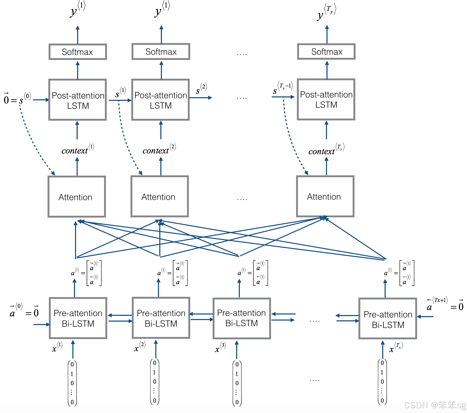
以下是你可能会注意到的模型的一些属性:
1)注意机制两侧的前注意和后注意lstm
2)LSTM同时具有隐藏状态和单元状态
3)每个时间步并不使用前一个时间步的预测
- * 与课程前面的文本生成示例不同,在这个模型中,时间$t$的后关注LSTM不将前一个时间步长的预测
 作为输入。
作为输入。 - * 后注意LSTM在时刻‘t’只接受隐藏状态
 和单元格状态
 作为输入。
作为输入。 - * 我们这样设计模型是因为与语言生成(相邻字符高度相关)不同,在YYYY-MM-DD日期中,前一个字符和下一个字符之间没有那么强的依赖性。
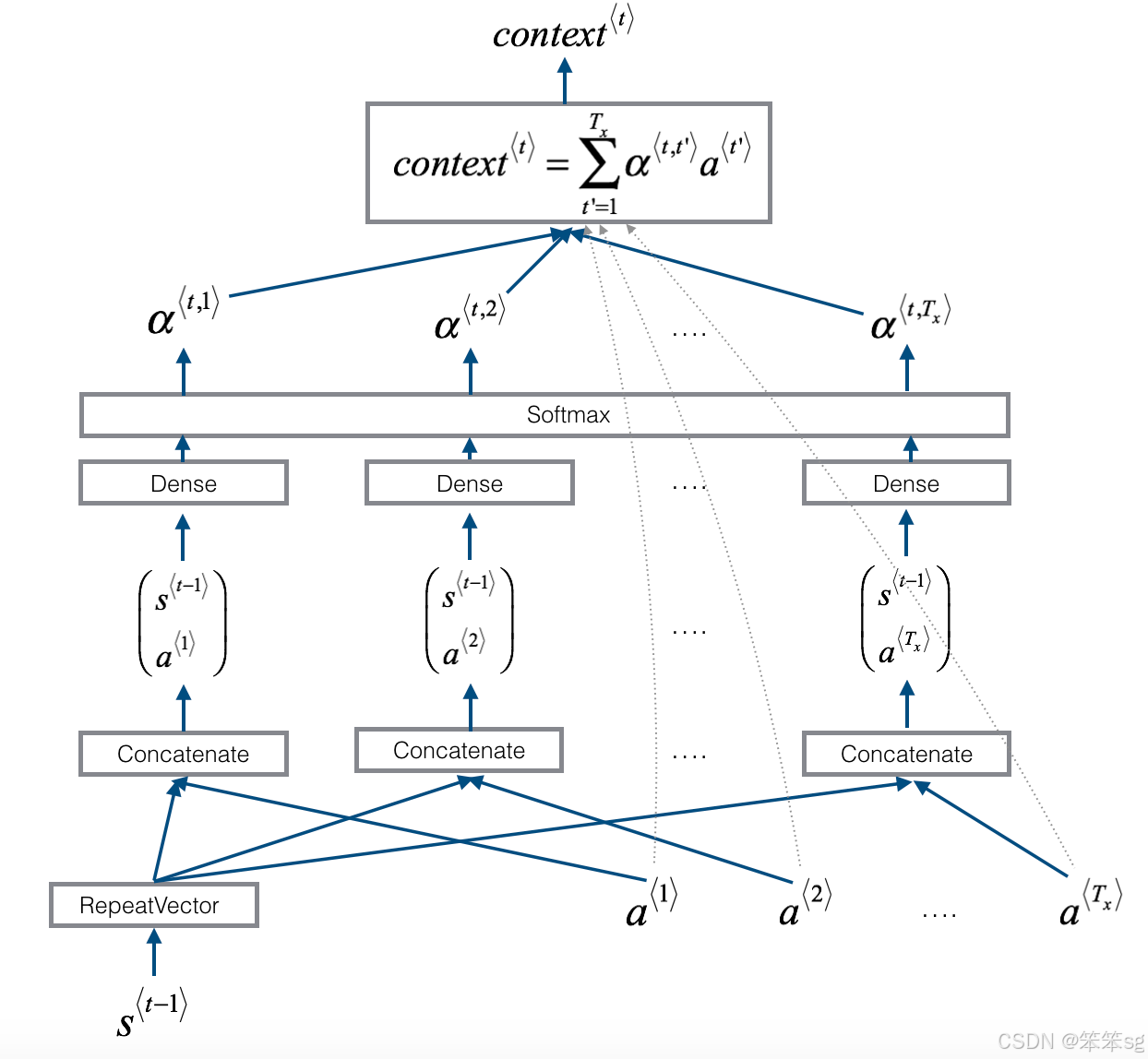
one_step_attention
- # Defined shared layers as global variables
- repeator = RepeatVector(Tx)
- concatenator = Concatenate(axis=-1)
- densor1 = Dense(10, activation = "tanh")
- densor2 = Dense(1, activation = "relu")
- activator = Activation(softmax, name='attention_weights') # We are using a custom softmax(axis = 1) loaded in this notebook
- dotor = Dot(axes = 1)
- # UNQ_C1 (UNIQUE CELL IDENTIFIER, DO NOT EDIT)
- # GRADED FUNCTION: one_step_attention
-
- def one_step_attention(a, s_prev):
-
- # Use repeator to repeat s_prev to be of shape (m, Tx, n_s) so that you can concatenate it with all hidden states "a" (≈ 1 line)
- s_prev = repeator(s_prev)
- # Use concatenator to concatenate a and s_prev on the last axis (≈ 1 line)
- # For grading purposes, please list 'a' first and 's_prev' second, in this order.
- concat = concatenator([a,s_prev])
- # Use densor1 to propagate concat through a small fully-connected neural network to compute the "intermediate energies" variable e. (≈1 lines)
- e = densor1(concat)
- # Use densor2 to propagate e through a small fully-connected neural network to compute the "energies" variable energies. (≈1 lines)
- energies = densor2(e)
- # Use "activator" on "energies" to compute the attention weights "alphas" (≈ 1 line)
- alphas = activator(energies)
- # Use dotor together with "alphas" and "a", in this order, to compute the context vector to be given to the next (post-attention) LSTM-cell (≈ 1 line)
- context = dotor([alphas,a])
-
- return context
- from tensorflow.python import framework as myframework
- # UNIT TEST
- def one_step_attention_test(target):
-
- m = 10
- Tx = 30
- n_a = 32
- n_s = 64
- #np.random.seed(10)
- a = np.random.uniform(1, 0, (m, Tx, 2 * n_a)).astype(np.float32)
- s_prev =np.random.uniform(1, 0, (m, n_s)).astype(np.float32) * 1
- context = target(a, s_prev)
-
- assert type(context) == myframework.ops.EagerTensor, "Unexpected type. It should be a Tensor"
- assert tuple(context.shape) == (m, 1, n_s), "Unexpected output shape"
- assert np.all(context.numpy() > 0), "All output values must be > 0 in this example"
- assert np.all(context.numpy() < 1), "All output values must be < 1 in this example"
-
- #assert np.allclose(context[0][0][0:5].numpy(), [0.50877404, 0.57160693, 0.45448175, 0.50074816, 0.53651875]), "Unexpected values in the result"
- print("\033[92mAll tests passed!")
-
- one_step_attention_test(one_step_attention)
All tests passed!
modelf
- n_a = 32 # number of units for the pre-attention, bi-directional LSTM's hidden state 'a'
- n_s = 64 # number of units for the post-attention LSTM's hidden state "s"
-
- # Please note, this is the post attention LSTM cell.
- post_activation_LSTM_cell = LSTM(n_s, return_state = True) # Please do not modify this global variable.
- output_layer = Dense(len(machine_vocab), activation=softmax)
- # UNQ_C2 (UNIQUE CELL IDENTIFIER, DO NOT EDIT)
- # GRADED FUNCTION: model
-
- def modelf(Tx, Ty, n_a, n_s, human_vocab_size, machine_vocab_size):
-
- # Define the inputs of your model with a shape (Tx,)
- # Define s0 (initial hidden state) and c0 (initial cell state)
- # for the decoder LSTM with shape (n_s,)
- X = Input(shape=(Tx, human_vocab_size))
- s0 = Input(shape=(n_s,), name='s0')
- c0 = Input(shape=(n_s,), name='c0')
- s = s0
- c = c0
-
- # Initialize empty list of outputs
- outputs = []
-
- # Step 1: Define your pre-attention Bi-LSTM. (≈ 1 line)
- a = Bidirectional(LSTM(n_a, return_sequences=True))(X)
-
- # Step 2: Iterate for Ty steps
- for t in range(Ty):
-
- # Step 2.A: Perform one step of the attention mechanism to get back the context vector at step t (≈ 1 line)
- context = one_step_attention(a, s)
-
- # Step 2.B: Apply the post-attention LSTM cell to the "context" vector.
- # Don't forget to pass: initial_state = [hidden state, cell state] (≈ 1 line)
- s, _, c = post_activation_LSTM_cell(context,initial_state=[s, c])
-
- # Step 2.C: Apply Dense layer to the hidden state output of the post-attention LSTM (≈ 1 line)
- out = output_layer(s)
-
- # Step 2.D: Append "out" to the "outputs" list (≈ 1 line)
- outputs.append(out)
-
- # Step 3: Create model instance taking three inputs and returning the list of outputs. (≈ 1 line)
- model = Model(inputs=[X, s0, c0],outputs=outputs)
-
- return model
- # UNIT TEST
- from test_utils import *
-
- def modelf_test(target):
- m = 10
- Tx = 30
- n_a = 32
- n_s = 64
- len_human_vocab = 37
- len_machine_vocab = 11
-
-
- model = target(Tx, Ty, n_a, n_s, len_human_vocab, len_machine_vocab)
-
- print(summary(model))
-
-
- expected_summary = [['InputLayer', [(None, 30, 37)], 0],
- ['InputLayer', [(None, 64)], 0],
- ['Bidirectional', (None, 30, 64), 17920],
- ['RepeatVector', (None, 30, 64), 0, 30],
- ['Concatenate', (None, 30, 128), 0],
- ['Dense', (None, 30, 10), 1290, 'tanh'],
- ['Dense', (None, 30, 1), 11, 'relu'],
- ['Activation', (None, 30, 1), 0],
- ['Dot', (None, 1, 64), 0],
- ['InputLayer', [(None, 64)], 0],
- ['LSTM',[(None, 64), (None, 64), (None, 64)], 33024,[(None, 1, 64), (None, 64), (None, 64)],'tanh'],
- ['Dense', (None, 11), 715, 'softmax']]
-
- comparator(summary(model), expected_summary)
-
-
- modelf_test(modelf)
[['InputLayer', [(None, 30, 37)], 0], ['InputLayer', [(None, 64)], 0], ['Bidirectional', (None, 30, 64), 17920], ['RepeatVector', (None, 30, 64), 0, 30], ['Concatenate', (None, 30, 128), 0], ['Dense', (None, 30, 10), 1290, 'tanh'], ['Dense', (None, 30, 1), 11, 'relu'], ['Activation', (None, 30, 1), 0], ['Dot', (None, 1, 64), 0], ['InputLayer', [(None, 64)], 0], ['LSTM', [(None, 64), (None, 64), (None, 64)], 33024, [(None, 1, 64), (None, 64), (None, 64)], 'tanh'], ['Dense', (None, 11), 715, 'softmax']]
All tests passed!
model = modelf(Tx, Ty, n_a, n_s, len(human_vocab), len(machine_vocab))让我们获取模型的摘要,以检查它是否与预期输出匹配。
model.summary()- Model: "model_1"
- __________________________________________________________________________________________________
- Layer (type) Output Shape Param # Connected to
- ==================================================================================================
- input_2 (InputLayer) [(None, 30, 37)] 0
- __________________________________________________________________________________________________
- s0 (InputLayer) [(None, 64)] 0
- __________________________________________________________________________________________________
- bidirectional_1 (Bidirectional) (None, 30, 64) 17920 input_2[0][0]
- __________________________________________________________________________________________________
- repeat_vector (RepeatVector) (None, 30, 64) 0 s0[0][0]
- lstm[10][0]
- lstm[11][0]
- lstm[12][0]
- lstm[13][0]
- lstm[14][0]
- lstm[15][0]
- lstm[16][0]
- lstm[17][0]
- lstm[18][0]
- __________________________________________________________________________________________________
- concatenate (Concatenate) (None, 30, 128) 0 bidirectional_1[0][0]
- repeat_vector[10][0]
- bidirectional_1[0][0]
- repeat_vector[11][0]
- bidirectional_1[0][0]
- repeat_vector[12][0]
- bidirectional_1[0][0]
- repeat_vector[13][0]
- bidirectional_1[0][0]
- repeat_vector[14][0]
- bidirectional_1[0][0]
- repeat_vector[15][0]
- bidirectional_1[0][0]
- repeat_vector[16][0]
- bidirectional_1[0][0]
- repeat_vector[17][0]
- bidirectional_1[0][0]
- repeat_vector[18][0]
- bidirectional_1[0][0]
- repeat_vector[19][0]
- __________________________________________________________________________________________________
- dense (Dense) (None, 30, 10) 1290 concatenate[10][0]
- concatenate[11][0]
- concatenate[12][0]
- concatenate[13][0]
- concatenate[14][0]
- concatenate[15][0]
- concatenate[16][0]
- concatenate[17][0]
- concatenate[18][0]
- concatenate[19][0]
- __________________________________________________________________________________________________
- dense_1 (Dense) (None, 30, 1) 11 dense[10][0]
- dense[11][0]
- dense[12][0]
- dense[13][0]
- dense[14][0]
- dense[15][0]
- dense[16][0]
- dense[17][0]
- dense[18][0]
- dense[19][0]
- __________________________________________________________________________________________________
- attention_weights (Activation) (None, 30, 1) 0 dense_1[10][0]
- dense_1[11][0]
- dense_1[12][0]
- dense_1[13][0]
- dense_1[14][0]
- dense_1[15][0]
- dense_1[16][0]
- dense_1[17][0]
- dense_1[18][0]
- dense_1[19][0]
- __________________________________________________________________________________________________
- dot (Dot) (None, 1, 64) 0 attention_weights[10][0]
- bidirectional_1[0][0]
- attention_weights[11][0]
- bidirectional_1[0][0]
- attention_weights[12][0]
- bidirectional_1[0][0]
- attention_weights[13][0]
- bidirectional_1[0][0]
- attention_weights[14][0]
- bidirectional_1[0][0]
- attention_weights[15][0]
- bidirectional_1[0][0]
- attention_weights[16][0]
- bidirectional_1[0][0]
- attention_weights[17][0]
- bidirectional_1[0][0]
- attention_weights[18][0]
- bidirectional_1[0][0]
- attention_weights[19][0]
- bidirectional_1[0][0]
- __________________________________________________________________________________________________
- c0 (InputLayer) [(None, 64)] 0
- __________________________________________________________________________________________________
- lstm (LSTM) [(None, 64), (None, 33024 dot[10][0]
- s0[0][0]
- c0[0][0]
- dot[11][0]
- lstm[10][0]
- lstm[10][2]
- dot[12][0]
- lstm[11][0]
- lstm[11][2]
- dot[13][0]
- lstm[12][0]
- lstm[12][2]
- dot[14][0]
- lstm[13][0]
- lstm[13][2]
- dot[15][0]
- lstm[14][0]
- lstm[14][2]
- dot[16][0]
- lstm[15][0]
- lstm[15][2]
- dot[17][0]
- lstm[16][0]
- lstm[16][2]
- dot[18][0]
- lstm[17][0]
- lstm[17][2]
- dot[19][0]
- lstm[18][0]
- lstm[18][2]
- __________________________________________________________________________________________________
- dense_2 (Dense) (None, 11) 715 lstm[10][0]
- lstm[11][0]
- lstm[12][0]
- lstm[13][0]
- lstm[14][0]
- lstm[15][0]
- lstm[16][0]
- lstm[17][0]
- lstm[18][0]
- lstm[19][0]
- ==================================================================================================
- Total params: 52,960
- Trainable params: 52,960
- Non-trainable params: 0
- __________________________________________________________________________________________________
编译模型
- opt = Adam(lr=0.005, beta_1=0.9, beta_2=0.999, decay=0.01)
- model.compile(optimizer=opt, loss='categorical_crossentropy', metrics=['accuracy'])
- # UNIT TESTS
- assert opt.lr == 0.005, "Set the lr parameter to 0.005"
- assert opt.beta_1 == 0.9, "Set the beta_1 parameter to 0.9"
- assert opt.beta_2 == 0.999, "Set the beta_2 parameter to 0.999"
- assert opt.decay == 0.01, "Set the decay parameter to 0.01"
- assert model.loss == "categorical_crossentropy", "Wrong loss. Use 'categorical_crossentropy'"
- assert model.optimizer == opt, "Use the optimizer that you have instantiated"
- assert model.compiled_metrics._user_metrics[0] == 'accuracy', "set metrics to ['accuracy']"
-
- print("\033[92mAll tests passed!")
All tests passed!
定义输入和输出,然后训练模型
- s0 = np.zeros((m, n_s))
- c0 = np.zeros((m, n_s))
- outputs = list(Yoh.swapaxes(0,1))
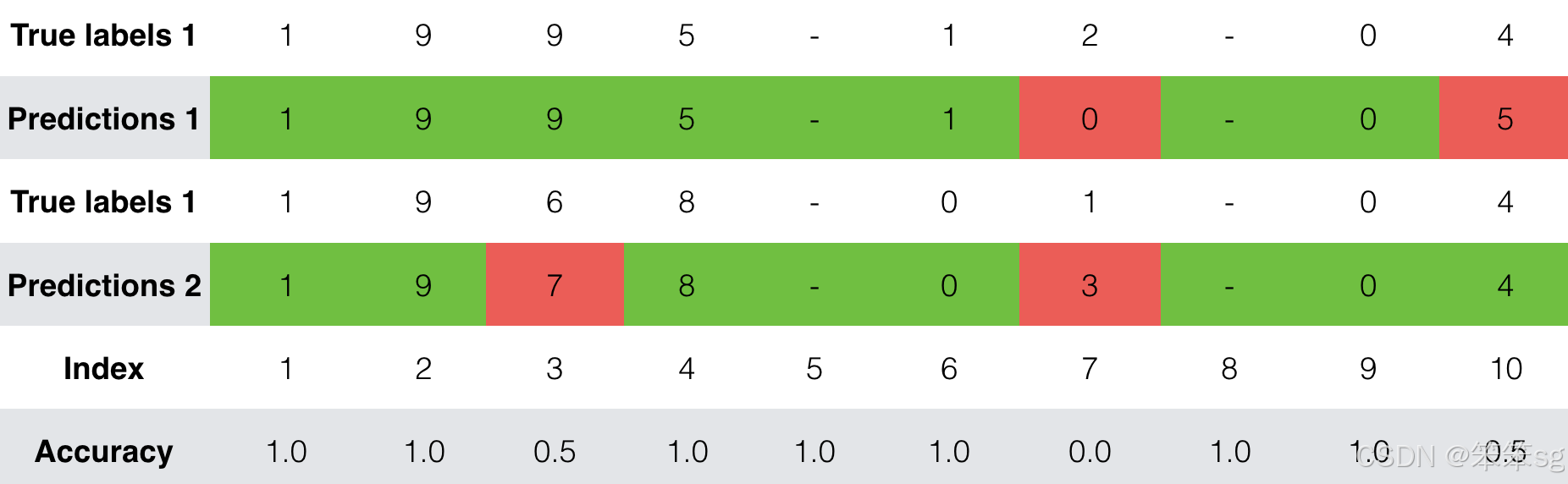
model.fit([Xoh, s0, c0], outputs, epochs=1, batch_size=100)100/100 [==============================] - 20s 49ms/step - loss: 19.9715 - dense_2_loss: 1.8134 - dense_2_1_loss: 1.6386 - dense_2_2_loss: 2.1659 - dense_2_3_loss: 2.7257 - dense_2_4_loss: 1.2834 - dense_2_5_loss: 1.6420 - dense_2_6_loss: 2.7552 - dense_2_7_loss: 1.3648 - dense_2_8_loss: 1.8986 - dense_2_9_loss: 2.6840 - dense_2_accuracy: 0.1713 - dense_2_1_accuracy: 0.4065 - dense_2_2_accuracy: 0.1710 - dense_2_3_accuracy: 0.0674 - dense_2_4_accuracy: 0.8328 - dense_2_5_accuracy: 0.1359 - dense_2_6_accuracy: 0.0128 - dense_2_7_accuracy: 0.8703 - dense_2_8_accuracy: 0.1518 - dense_2_9_accuracy: 0.0724
在训练时,您可以看到输出的10个位置中的每个位置的损失和准确性。下表给出了一个例子,说明如果批处理有2个例子,准确度可能是多少:
我们运行这个模型的时间更长,并且保存了权重。运行下一个单元格来加载权重。(通过训练模型几分钟,您应该能够获得类似精度的模型,但加载我们的模型将节省您的时间。)
model.load_weights('models/model.h5')现在可以在新的示例上看到结果。
- EXAMPLES = ['3 May 1979', '5 April 09', '21th of August 2016', 'Tue 10 Jul 2007', 'Saturday May 9 2018', 'March 3 2001', 'March 3rd 2001', '1 March 2001']
- s00 = np.zeros((1, n_s))
- c00 = np.zeros((1, n_s))
- for example in EXAMPLES:
- source = string_to_int(example, Tx, human_vocab)
- #print(source)
- source = np.array(list(map(lambda x: to_categorical(x, num_classes=len(human_vocab)), source))).swapaxes(0,1)
- source = np.swapaxes(source, 0, 1)
- source = np.expand_dims(source, axis=0)
- prediction = model.predict([source, s00, c00])
- prediction = np.argmax(prediction, axis = -1)
- output = [inv_machine_vocab[int(i)] for i in prediction]
- print("source:", example)
- print("output:", ''.join(output),"\n")
source: 3 May 1979
output: 1979-05-33source: 5 April 09
output: 2009-04-05source: 21th of August 2016
output: 2016-08-20source: Tue 10 Jul 2007
output: 2007-07-10source: Saturday May 9 2018
output: 2018-05-09source: March 3 2001
output: 2001-03-03source: March 3rd 2001
output: 2001-03-03source: 1 March 2001
output: 2001-03-01
- def translate_date(sentence):
- source = string_to_int(sentence, Tx, human_vocab)
- source = np.array(list(map(lambda x: to_categorical(x, num_classes=len(human_vocab)), source))).swapaxes(0,1)
- source = np.swapaxes(source, 0, 1)
- source = np.expand_dims(source, axis=0)
- prediction = model.predict([source, s00, c00])
- prediction = np.argmax(prediction, axis = -1)
- output = [inv_machine_vocab[int(i)] for i in prediction]
- print("source:", sentence)
- print("output:", ''.join(output),"\n")
- example = "4th of july 2001"
- translate_date(example)
source: 4th of july 2001
output: 2001-07-04
您还可以更改这些示例,以便用您自己的示例进行测试。下一部分会让你更好地理解注意力机制的作用。当生成一个特定的输出字符时,网络关注的是输入的哪个部分。
2.4 可视化注意力
由于问题的输出长度固定为10,因此也可以使用10个不同的softmax单元来生成输出的10个字符来执行此任务。但是注意力模型的一个优点是,输出的每个部分(比如月份)都知道它只需要依赖于输入的一小部分(输入中给出月份的字符)。我们可以看到输出的每一部分在看输入的哪一部分。
考虑将"Saturday 9 May 2018"翻译为“2018-05-09”的任务。如果我们把计算 我们可以得到:
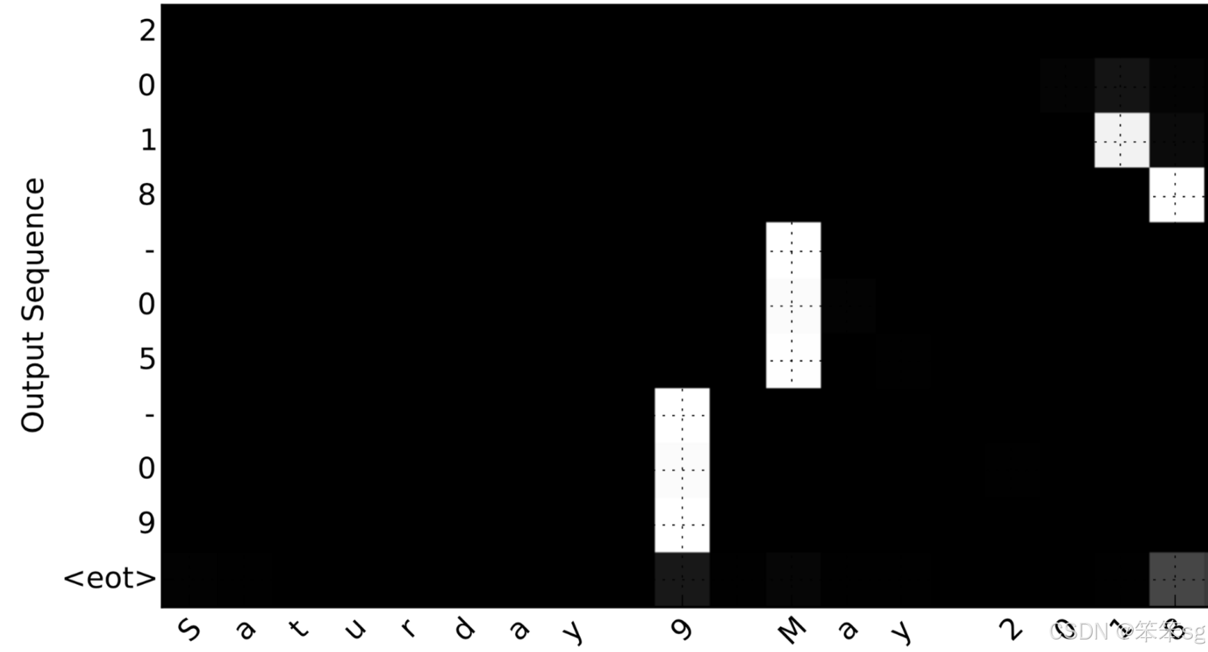
注意输出是如何忽略输入的“Saturday”部分的。所有的输出时间步都不太关注这部分输入。我们还看到9被翻译成了09,May被正确地翻译成了05,输出注意到了输入中需要翻译的部分。年主要要求它注意输入的“18”,以便生成“2018”。"
从网络中获取注意力权重
现在让我们可视化你的网络中的注意力值。我们将通过网络传播一个示例,然后可视化的值。
为了找出注意力值的位置,让我们从打印模型摘要开始。
model.summary()- Model: "model_1"
- __________________________________________________________________________________________________
- Layer (type) Output Shape Param # Connected to
- ==================================================================================================
- input_2 (InputLayer) [(None, 30, 37)] 0
- __________________________________________________________________________________________________
- s0 (InputLayer) [(None, 64)] 0
- __________________________________________________________________________________________________
- bidirectional_1 (Bidirectional) (None, 30, 64) 17920 input_2[0][0]
- __________________________________________________________________________________________________
- repeat_vector (RepeatVector) (None, 30, 64) 0 s0[0][0]
- lstm[10][0]
- lstm[11][0]
- lstm[12][0]
- lstm[13][0]
- lstm[14][0]
- lstm[15][0]
- lstm[16][0]
- lstm[17][0]
- lstm[18][0]
- __________________________________________________________________________________________________
- concatenate (Concatenate) (None, 30, 128) 0 bidirectional_1[0][0]
- repeat_vector[10][0]
- bidirectional_1[0][0]
- repeat_vector[11][0]
- bidirectional_1[0][0]
- repeat_vector[12][0]
- bidirectional_1[0][0]
- repeat_vector[13][0]
- bidirectional_1[0][0]
- repeat_vector[14][0]
- bidirectional_1[0][0]
- repeat_vector[15][0]
- bidirectional_1[0][0]
- repeat_vector[16][0]
- bidirectional_1[0][0]
- repeat_vector[17][0]
- bidirectional_1[0][0]
- repeat_vector[18][0]
- bidirectional_1[0][0]
- repeat_vector[19][0]
- __________________________________________________________________________________________________
- dense (Dense) (None, 30, 10) 1290 concatenate[10][0]
- concatenate[11][0]
- concatenate[12][0]
- concatenate[13][0]
- concatenate[14][0]
- concatenate[15][0]
- concatenate[16][0]
- concatenate[17][0]
- concatenate[18][0]
- concatenate[19][0]
- __________________________________________________________________________________________________
- dense_1 (Dense) (None, 30, 1) 11 dense[10][0]
- dense[11][0]
- dense[12][0]
- dense[13][0]
- dense[14][0]
- dense[15][0]
- dense[16][0]
- dense[17][0]
- dense[18][0]
- dense[19][0]
- __________________________________________________________________________________________________
- attention_weights (Activation) (None, 30, 1) 0 dense_1[10][0]
- dense_1[11][0]
- dense_1[12][0]
- dense_1[13][0]
- dense_1[14][0]
- dense_1[15][0]
- dense_1[16][0]
- dense_1[17][0]
- dense_1[18][0]
- dense_1[19][0]
- __________________________________________________________________________________________________
- dot (Dot) (None, 1, 64) 0 attention_weights[10][0]
- bidirectional_1[0][0]
- attention_weights[11][0]
- bidirectional_1[0][0]
- attention_weights[12][0]
- bidirectional_1[0][0]
- attention_weights[13][0]
- bidirectional_1[0][0]
- attention_weights[14][0]
- bidirectional_1[0][0]
- attention_weights[15][0]
- bidirectional_1[0][0]
- attention_weights[16][0]
- bidirectional_1[0][0]
- attention_weights[17][0]
- bidirectional_1[0][0]
- attention_weights[18][0]
- bidirectional_1[0][0]
- attention_weights[19][0]
- bidirectional_1[0][0]
- __________________________________________________________________________________________________
- c0 (InputLayer) [(None, 64)] 0
- __________________________________________________________________________________________________
- lstm (LSTM) [(None, 64), (None, 33024 dot[10][0]
- s0[0][0]
- c0[0][0]
- dot[11][0]
- lstm[10][0]
- lstm[10][2]
- dot[12][0]
- lstm[11][0]
- lstm[11][2]
- dot[13][0]
- lstm[12][0]
- lstm[12][2]
- dot[14][0]
- lstm[13][0]
- lstm[13][2]
- dot[15][0]
- lstm[14][0]
- lstm[14][2]
- dot[16][0]
- lstm[15][0]
- lstm[15][2]
- dot[17][0]
- lstm[16][0]
- lstm[16][2]
- dot[18][0]
- lstm[17][0]
- lstm[17][2]
- dot[19][0]
- lstm[18][0]
- lstm[18][2]
- __________________________________________________________________________________________________
- dense_2 (Dense) (None, 11) 715 lstm[10][0]
- lstm[11][0]
- lstm[12][0]
- lstm[13][0]
- lstm[14][0]
- lstm[15][0]
- lstm[16][0]
- lstm[17][0]
- lstm[18][0]
- lstm[19][0]
- ==================================================================================================
- Total params: 52,960
- Trainable params: 52,960
- Non-trainable params: 0
- __________________________________________________________________________________________________
浏览上面‘ model.summary() ’的输出。你可以看到,名为 `attention_weights`的层在`alphas`计算每个时间步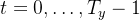 之前,输出形状(m, 30,1)的‘ alpha ’。让我们从这一层得到注意力权重。
函数‘ attention_map() ’从模型中提取注意力值并绘制它们。
attention_map = plot_attention_map(model, human_vocab, inv_machine_vocab, "Tuesday 09 Oct 1993", num = 7, n_s = 64);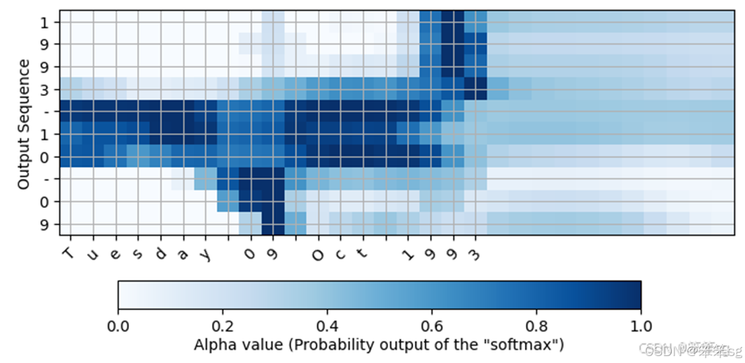
在生成的图上,您可以观察到预测输出的每个字符的注意权重值。检查这张图,并检查网络关注的地方是否对你有意义。
在日期翻译应用程序中,您将观察到大多数时间注意力有助于预测年份,而对预测日期或月份没有太大影响。
恭喜你!你的任务已经完成了
下面是你应该记住的:
- - 机器翻译模型可用于从一个序列映射到另一个序列。它们不仅适用于翻译人类语言(如法语->英语),也适用于日期格式翻译等任务。
- - 注意机制允许网络在产生输出的特定部分时专注于输入中最相关的部分。
- - 使用注意机制的网络可以从长度
的输入转换为长度
的输出,其中
- - 你可以可视化注意力权重
,以查看网络在生成每个输出时关注的内容。
祝贺你完成了这个作业!现在,您可以实现一个注意力模型,并使用它来学习从一个序列到另一个序列的复杂映射。
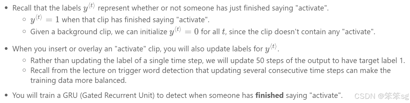
3 触发词检测
欢迎来到第三周的第二个也是最后一个编程作业!
在本周的视频中,你学习了如何将深度学习应用于语音识别。在本作业中,您将构建一个语音数据集并实现触发词检测(有时也称为关键字检测或唤醒词检测)的算法。
- * 触发词检测是一项技术,允许亚马逊Alexa、b谷歌Home、苹果Siri和百度DuerOS等设备在听到某个单词时醒来。
- * 在这个练习中,我们的触发词是“activate”。每次听到你说“激活”,它就会发出“报时”的声音。
- * 在这项任务结束时,你将能够录制自己说话的片段,并让算法在检测到你说“激活”时触发铃声。
- * 完成这个任务后,也许你也可以扩展它在你的笔记本电脑上运行,这样每次你说“激活”,它就会启动你最喜欢的应用程序,或者打开你家里的网络连接灯,或者触发其他一些事件?
在本作业中,你将学习:
- - 构建一个语音识别项目
- - 合成和处理音频记录,以创建训练/开发数据集
- - 训练触发词检测模型并进行预测
让我们开始吧!
3.0 导包
- import numpy as np
- from pydub import AudioSegment
- import tensorflow as tf
- import random
- import sys
- import io
- import os
- import glob
- import IPython
- from td_utils import *
- # 解决模型加载显存占满的问题
- physical_gpus = tf.config.list_physical_devices("GPU")
- tf.config.experimental.set_memory_growth(physical_gpus[0], True)
- logical_gpus = tf.config.list_logical_devices("GPU")
-
- %matplotlib inline
3.1 数据合成:创建语言数据集
让我们首先为您的触发词检测算法构建一个数据集。
- * 理想情况下,语音数据集应该尽可能接近你想要运行它的应用程序。
- * 在这种情况下,你想在工作环境(图书馆,家里,办公室,开放空间…)中检测单词“activate”。
- * 因此,你需要在不同的背景声音中混合积极的词("activate")和消极的词(除了激活之外的随机词)来创建录音。让我们看看如何创建这样的数据集。
聆听数据
- * 你的一个朋友正在帮助你完成这个项目,他们已经去了图书馆、咖啡馆、餐馆、家庭和办公室的所有区域,以记录背景噪音,以及人们说positive/negative的话的音频片段。这个数据集包括用各种口音说话的人。
- * 在raw_data目录中,您可以找到积极词、消极词和背景噪声的原始音频文件的子集。您将使用这些音频文件合成一个数据集来训练模型。
- * “activate”目录包含人们说“activate”这个词的积极例子。
- * “negatives”目录包含否定的例子,人们说随机单词,而不是“activate”。
- *每个音频记录有一个单词。
- * “backgrounds”目录包含10秒的背景噪音剪辑在不同的环境。
运行下面的单元格来听一些例子。
IPython.display.Audio("./raw_data/activates/1.wav")![]()
您将使用这三种类型的记录(positives/negatives/backgrounds)来创建标记的数据集。
从录音到频谱图
1)录音到底是什么?
- * 麦克风会记录气压随时间的微小变化,而你的耳朵也会将这些气压的微小变化感知为声音。
- * 你可以把录音想象成一长串数字,用来测量麦克风检测到的气压变化。
- * 我们将使用44100 Hz(或44100赫兹)的音频采样。
- * 这意味着麦克风每秒输出44100个数字。
- * 因此,一个10秒的音频片段由441,000个数字表示(=
 ).
).
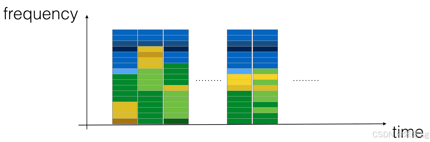
2)频谱图
- * 很难从音频的“原始”表示中判断是否说了单词“activate”。
- * 为了帮助你的序列模型更容易地学习检测触发词,我们将计算音频的频谱图。
- * 频谱图告诉我们在任何时刻音频片段中存在多少不同的频率。
- * 如果你上过信号处理或傅里叶变换的高级课程:
- * 频谱图是通过在原始音频信号上滑动窗口来计算的,并使用傅里叶变换计算每个窗口中最活跃的频率。
- * 如果你不明白前面的句子,不要担心。让我们来看一个例子。
x = graph_spectrogram("audio_examples/example_train.wav")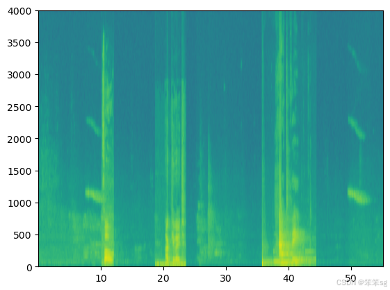
上面的图表表示每个频率(y轴)在多个时间步长(x轴)上的活跃程度。
- * 频谱图中的颜色表示在不同时间点音频中不同频率存在的程度(大声)。
- * 绿色表示某个频率更活跃或在音频片段中更存在(更大声)。
- * 蓝色方块表示较低的活跃频率。
- * 输出谱图的尺寸取决于谱图软件的超参数和输入的长度。
- * 在本笔记本中,我们将使用10秒音频剪辑作为我们训练示例的“标准长度”。
- * 频谱图的时间步长为5511。
- * 稍后您将看到,频谱图将是网络的输入
 ,因此
,因此 。
。
- _, data = wavfile.read("audio_examples/example_train.wav")
- print("Time steps in audio recording before spectrogram", data[:,0].shape)
- print("Time steps in input after spectrogram", x.shape)
Time steps in audio recording before spectrogram (441000,)
Time steps in input after spectrogram (101, 5511)
现在,你可以定义:
- Tx = 5511 # 从谱图输入到模型的时间步长数
- n_freq = 101 # 在频谱图的每个时间步输入到模型的频率数
3)划分时间间隔
- 注意,我们可以用不同的单位(步)来划分10秒的时间间隔。
- * 原始音频将10秒分成441,000个单位。
- * 谱图将10秒分成5511个单位。
- *
- * 您将使用Python模块‘ pydub ’来合成音频,它将10秒分成10,000个单元。
- * 我们型号的输出将把10秒分成1375个单位。
- *

- * 对于1375个时间步骤中的每一个,该模型预测某人最近是否说出了触发词“activate”。
- * 所有这些都是超参数,可以更改(441000除外,这是麦克风的功能)。
- * 我们选择的值在语音系统使用的标准范围内。
Ty = 1375 # 我们模型输出的时间步数综合数据的好处
* 由于语音数据很难获取和标记,因此您将使用positives/negatives/backgrounds的音频剪辑来合成您的训练数据。
* 当有随机“positives”在时记录大量的10秒音频剪辑是相当慢的。
* 相反,更容易记录大量的positive和negative的单词,并记录background噪音(或从免费的在线资源下载背景噪音)。
合成音频剪辑的过程
* 要综合单个训练示例,您将:
- 选择一个随机的10秒背景音频剪辑
- 随机插入0-4音频剪辑“activate”到这个10秒的剪辑
- 随机插入0-2个"negative"的音频剪辑到这个10秒的剪辑
* 因为你已经将单词“activate”合成到背景剪辑中,你知道在10秒剪辑中“activate”出现的确切时间。
稍后您将看到,这也使得生成标签
变得更加容易。
Pydub
* 您将使用pydub包来操作音频。
* Pydub将原始音频文件转换为Pydub数据结构列表。
* 不要担心数据结构的细节。
* Pydub使用1ms作为离散间隔(1ms = 1毫秒= 1/1000秒)。
* 这就是为什么一个10秒的剪辑总是用10000步来表示。
- # Load audio segments using pydub
- activates, negatives, backgrounds = load_raw_audio('./raw_data/')
-
- print("background len should be 10,000, since it is a 10 sec clip\n" + str(len(backgrounds[0])),"\n")
- print("activate[0] len may be around 1000, since an `activate` audio clip is usually around 1 second (but varies a lot) \n" + str(len(activates[0])),"\n")
- print("activate[1] len: different `activate` clips can have different lengths\n" + str(len(activates[1])),"\n")
background len should be 10,000, since it is a 10 sec clip
10000activate[0] len may be around 1000, since an `activate` audio clip is usually around 1 second (but varies a lot)
721activate[1] len: different `activate` clips can have different lengths
731
生成单个训练样例
1)叠加positives/negatives的“单词”音频剪辑在背景音频的顶部
- * 给定一个10秒的背景剪辑和一个简短的音频剪辑包含一个积极或消极的词,你需要能够“添加”单词音频剪辑在背景音频的顶部。
- * 你将插入多个剪辑的积极/消极的单词到背景中,你不想插入一个“激活”或一个随机的单词,与你之前添加的另一个剪辑重叠的地方。
- * 为了确保“word”音频段在插入时不重叠,您将跟踪以前插入的音频剪辑的时间。
- * 要明确的是,当你插入一个1秒的“激活”到一个10秒的咖啡馆噪音剪辑,你不会以一个11秒的剪辑结束
- * 产生的音频剪辑仍然是10秒长。
- * 稍后您将看到pydub如何允许您这样做。
2)给积极/消极的词语贴上标签
例子:
合成数据更容易标记
- * 这是合成训练数据的另一个原因:如上所述,生成这些标签$y^{\langle t \rangle}$相对简单。
- * 相比之下,如果你在麦克风上录制了10秒的音频,那么对于一个人来说,听它并手动标记“激活”完成的时间是非常耗时的。
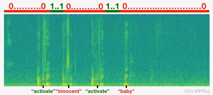
3)可视化标签
* 这张图说明了一个剪辑中的标签。
* 我们插入了“activate”, “innocent”, “activate”, “baby ”。
* 注意,积极的标签“1”只与积极的单词相关联。
4)辅助函数
要实现训练集合成过程,您将使用以下辅助函数。
* 所有这些函数将使用1ms的离散间隔
* 10秒的音频总是离散成10000步。
1. `get_random_time_segment(segment_ms)`
* 从背景音频中检索随机时间段。
2. `is_overlapping(segment_time, existing_segments)`
* 检查一个时间段是否与现有的时间段重叠
3. `insert_audio_clip(background, audio_clip, existing_times)`
* 插入一个音频段在一个随机的时间在背景音频
* 使用函数 `get_random_time_segment` and `is_overlapping`
4. `insert_ones(y, segment_end_ms)`
* 在单词“激活”后的标签向量y中插入额外的1
5)获取随机时间段
* 函数‘ get_random_time_segment(segment_ms) ’返回一个随机时间段,我们可以插入一个持续时间‘ segment_ms ’的音频剪辑。
* 请通读代码以确保你明白它在做什么。
- def get_random_time_segment(segment_ms):
- """
- Gets a random time segment of duration segment_ms in a 10,000 ms audio clip.
-
- Arguments:
- segment_ms -- the duration of the audio clip in ms ("ms" stands for "milliseconds")
-
- Returns:
- segment_time -- a tuple of (segment_start, segment_end) in ms
- """
-
- segment_start = np.random.randint(low=0, high=10000-segment_ms) # Make sure segment doesn't run past the 10sec background
- segment_end = segment_start + segment_ms - 1
-
- return (segment_start, segment_end)
6)检查音频剪辑是否重叠
* 假设您在片段(1000,1800)和片段(3400,4500)插入了音频剪辑。
* 第一个片段从第1000步开始,到第1800步结束。
* 第二段从3400开始,到4500结束。
* 如果我们正在考虑是否在(3000,3600)插入一个新的音频剪辑,这是否与之前插入的片段重叠?
* 在这种情况下,(3000,3600)和(3400,4500)重叠,所以我们应该决定不插入剪辑在这里。
* 为了这个函数的目的,定义(100,200)和(200,250)是重叠的,因为它们在时间步长200重叠。
* (100,199)和(200,250)不重叠。
- # UNQ_C1
- # GRADED FUNCTION: is_overlapping
-
- def is_overlapping(segment_time, previous_segments):
- """
- Checks if the time of a segment overlaps with the times of existing segments.
-
- Arguments:
- segment_time -- a tuple of (segment_start, segment_end) for the new segment
- previous_segments -- a list of tuples of (segment_start, segment_end) for the existing segments
-
- Returns:
- True if the time segment overlaps with any of the existing segments, False otherwise
- """
-
- segment_start, segment_end = segment_time
-
- # Step 1: Initialize overlap as a "False" flag. (≈ 1 line)
- overlap = False
-
- # Step 2: loop over the previous_segments start and end times.
- # Compare start/end times and set the flag to True if there is an overlap (≈ 3 lines)
- for previous_start, previous_end in previous_segments: # @KEEP
- if segment_start <= previous_end and segment_end >= previous_start:
- overlap = True
- break
-
- return overlap
- # UNIT TEST
- def is_overlapping_test(target):
- assert target((670, 1430), []) == False, "Overlap with an empty list must be False"
- assert target((500, 1000), [(100, 499), (1001, 1100)]) == False, "Almost overlap, but still False"
- assert target((750, 1250), [(100, 750), (1001, 1100)]) == True, "Must overlap with the end of first segment"
- assert target((750, 1250), [(300, 600), (1250, 1500)]) == True, "Must overlap with the begining of second segment"
- assert target((750, 1250), [(300, 600), (600, 1500), (1600, 1800)]) == True, "Is contained in second segment"
- print("\033[92m All tests passed!")
-
- is_overlapping_test(is_overlapping)
All tests passed!
- overlap1 = is_overlapping((950, 1430), [(2000, 2550), (260, 949)])
- overlap2 = is_overlapping((2305, 2950), [(824, 1532), (1900, 2305), (3424, 3656)])
- print("Overlap 1 = ", overlap1)
- print("Overlap 2 = ", overlap2)
Overlap 1 = False
Overlap 2 = True
7)插入音频剪辑
* 让我们使用前面的辅助函数在随机时间插入一个新的音频剪辑到10秒的背景上。
* 我们将确保任何新插入的段不会与先前插入的段重叠。
- # UNQ_C2
- # GRADED FUNCTION: insert_audio_clip
-
- def insert_audio_clip(background, audio_clip, previous_segments):
- """
- Insert a new audio segment over the background noise at a random time step, ensuring that the
- audio segment does not overlap with existing segments.
-
- Arguments:
- background -- a 10 second background audio recording.
- audio_clip -- the audio clip to be inserted/overlaid.
- previous_segments -- times where audio segments have already been placed
-
- Returns:
- new_background -- the updated background audio
- """
-
- # Get the duration of the audio clip in ms
- segment_ms = len(audio_clip)
-
- # Step 1: Use one of the helper functions to pick a random time segment onto which to insert
- # the new audio clip. (≈ 1 line)
- segment_time = get_random_time_segment(segment_ms)
-
- # Step 2: Check if the new segment_time overlaps with one of the previous_segments. If so, keep
- # picking new segment_time at random until it doesn't overlap. To avoid an endless loop
- # we retry 5 times(≈ 2 lines)
- retry = 5 # @KEEP
- while is_overlapping(segment_time, previous_segments) and retry >= 0:
- segment_time = get_random_time_segment(segment_ms)
- retry = retry - 1
-
- # if last try is not overlaping, insert it to the background
- if not is_overlapping(segment_time, previous_segments):
- # Step 3: Append the new segment_time to the list of previous_segments (≈ 1 line)
- previous_segments.append(segment_time)
- # Step 4: Superpose audio segment and background
- new_background = background.overlay(audio_clip, position = segment_time[0])
- print(segment_time)
- else:
- print("Timeouted")
- new_background = background
- segment_time = (10000, 10000)
-
- return new_background, segment_time
- # UNIT TEST
- def insert_audio_clip_test(target):
- np.random.seed(5)
- audio_clip, segment_time = target(backgrounds[0], activates[0], [(0, 4400)])
- duration = segment_time[1] - segment_time[0]
- assert segment_time[0] > 4400, "Error: The audio clip is overlaping with the first segment"
- assert duration + 1 == len(activates[0]) , "The segment length must match the audio clip length"
- assert audio_clip != backgrounds[0] , "The audio clip must be different than the pure background"
-
- # Not possible to insert clip into background
- audio_clip, segment_time = target(backgrounds[0], activates[0], [(0, 9999)])
- assert segment_time[0] == 10000 and segment_time[1] == 10000, "Segment must match the out by max-retry mark"
- assert audio_clip == backgrounds[0], "output audio clip must be exactly the same input background"
-
- print("\033[92m All tests passed!")
-
- insert_audio_clip_test(insert_audio_clip)
(7286, 8006)
Timeouted
All tests passed!
- np.random.seed(5)
- audio_clip, segment_time = insert_audio_clip(backgrounds[0], activates[0], [(3790, 4400)])
- audio_clip.export("insert_test.wav", format="wav")
- print("Segment Time: ", segment_time)
- IPython.display.Audio("insert_test.wav")
(2915, 3635)
Segment Time: (2915, 3635)

- # Expected audio
- IPython.display.Audio("audio_examples/insert_reference.wav")
8)插入positive目标的标签
* 实现代码来更新标签
* 在下面的代码中,‘ y ’是一个‘(1,1375)’维度向量,因为
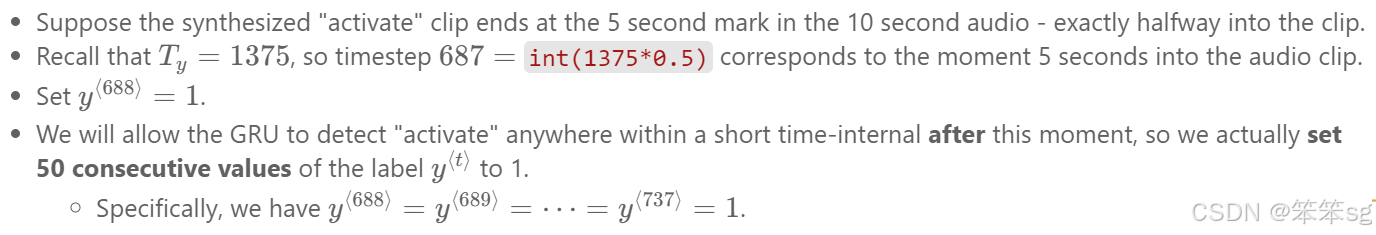
* 如果“激活”音频剪辑在时间步t结束,则设置
,并设置下一个49个额外的连续值为1。
* 请注意,如果目标单词出现在整个音频剪辑的末尾附近,则可能没有50个额外的时间步长设置为1。
* 确保你没有跑过数组的末尾并尝试更新‘ y[0][1375] ’,因为有效的索引是‘ y[0][0] ’到‘ y[0][1374] ’,因为
= 1375$。
* 如果“activate”在第1370步结束,你只会得到“y[0][1371] = y[0][1372] = y[0][1373] = y[0][1374] = 1”
- # UNQ_C3
- # GRADED FUNCTION: insert_ones
-
- def insert_ones(y, segment_end_ms):
- """
- Update the label vector y. The labels of the 50 output steps strictly after the end of the segment
- should be set to 1. By strictly we mean that the label of segment_end_y should be 0 while, the
- 50 following labels should be ones.
-
-
- Arguments:
- y -- numpy array of shape (1, Ty), the labels of the training example
- segment_end_ms -- the end time of the segment in ms
-
- Returns:
- y -- updated labels
- """
- _, Ty = y.shape
-
- # duration of the background (in terms of spectrogram time-steps)
- segment_end_y = int(segment_end_ms * Ty / 10000.0)
-
- if segment_end_y < Ty:
- # Add 1 to the correct index in the background label (y)
- for i in range(segment_end_y+1, segment_end_y+51):
- if i < Ty:
- y[0, i] = 1
-
- return y
- # UNIT TEST
- import random
- def insert_ones_test(target):
- segment_end_y = random.randrange(0, Ty - 50)
- segment_end_ms = int(segment_end_y * 10000.4) / Ty;
- arr1 = target(np.zeros((1, Ty)), segment_end_ms)
-
- assert type(arr1) == np.ndarray, "Wrong type. Output must be a numpy array"
- assert arr1.shape == (1, Ty), "Wrong shape. It must match the input shape"
- assert np.sum(arr1) == 50, "It must insert exactly 50 ones"
- assert arr1[0][segment_end_y - 1] == 0, f"Array at {segment_end_y - 1} must be 0"
- assert arr1[0][segment_end_y] == 0, f"Array at {segment_end_y} must be 1"
- assert arr1[0][segment_end_y + 1] == 1, f"Array at {segment_end_y + 1} must be 1"
- assert arr1[0][segment_end_y + 50] == 1, f"Array at {segment_end_y + 50} must be 1"
- assert arr1[0][segment_end_y + 51] == 0, f"Array at {segment_end_y + 51} must be 0"
-
- print("\033[92m All tests passed!")
-
- insert_ones_test(insert_ones)
All tests passed!
- arr1 = insert_ones(np.zeros((1, Ty)), 9700)
- plt.plot(insert_ones(arr1, 4251)[0,:])
- print("sanity checks:", arr1[0][1333], arr1[0][634], arr1[0][635])
sanity checks: 0.0 1.0 0.0
9)创建一个训练示例
最后,您可以使用‘ insert_audio_clip ’和‘ insert_ones ’来创建一个新的训练示例。
- # UNQ_C4
- # GRADED FUNCTION: create_training_example
-
- def create_training_example(background, activates, negatives, Ty):
- """
- Creates a training example with a given background, activates, and negatives.
-
- Arguments:
- background -- a 10 second background audio recording
- activates -- a list of audio segments of the word "activate"
- negatives -- a list of audio segments of random words that are not "activate"
- Ty -- The number of time steps in the output
- Returns:
- x -- the spectrogram of the training example
- y -- the label at each time step of the spectrogram
- """
-
- # Make background quieter
- background = background - 20
-
- # Step 1: Initialize y (label vector) of zeros (≈ 1 line)
- y = np.zeros((1, Ty))
-
- # Step 2: Initialize segment times as empty list (≈ 1 line)
- previous_segments = []
-
- # Select 0-4 random "activate" audio clips from the entire list of "activates" recordings
- number_of_activates = np.random.randint(0, 5)
- random_indices = np.random.randint(len(activates), size=number_of_activates)
- random_activates = [activates[i] for i in random_indices]
-
- # Step 3: Loop over randomly selected "activate" clips and insert in background
- for random_activate in random_activates: # @KEEP
- # Insert the audio clip on the background
- background, segment_time = insert_audio_clip(background, random_activate, previous_segments)
- # Retrieve segment_start and segment_end from segment_time
- segment_start, segment_end = segment_time
- # Insert labels in "y" at segment_end
- y = insert_ones(y, segment_end)
-
- # Select 0-2 random negatives audio recordings from the entire list of "negatives" recordings
- number_of_negatives = np.random.randint(0, 3)
- random_indices = np.random.randint(len(negatives), size=number_of_negatives)
- random_negatives = [negatives[i] for i in random_indices]
-
- # Step 4: Loop over randomly selected negative clips and insert in background
- for random_negative in random_negatives: # @KEEP
- # Insert the audio clip on the background
- background, _ = insert_audio_clip(background, random_negative, previous_segments)
-
- # Standardize the volume of the audio clip
- background = match_target_amplitude(background, -20.0)
-
- # Export new training example
- # file_handle = background.export("train" + ".wav", format="wav")
-
- # Get and plot spectrogram of the new recording (background with superposition of positive and negatives)
- x = graph_spectrogram("train.wav")
-
- return x, y
- # UNIT TEST
- def create_training_example_test(target):
- np.random.seed(18)
- x, y = target(backgrounds[0], activates, negatives, 1375)
-
- assert type(x) == np.ndarray, "Wrong type for x"
- assert type(y) == np.ndarray, "Wrong type for y"
- assert tuple(x.shape) == (101, 5511), "Wrong shape for x"
- assert tuple(y.shape) == (1, 1375), "Wrong shape for y"
- assert np.all(x > 0), "All x values must be higher than 0"
- assert np.all(y >= 0), "All y values must be higher or equal than 0"
- assert np.all(y < 51), "All y values must be smaller than 51"
- assert np.sum(y) % 50 == 0, "Sum of activate marks must be a multiple of 50"
- assert np.isclose(np.linalg.norm(x), 39745552.52075), "Spectrogram is wrong. Check the parameters passed to the insert_audio_clip function"
-
- print("\033[92m All tests passed!")
-
- create_training_example_test(create_training_example)
(2885, 3793)
(5294, 7685)
(9105, 9511)
(645, 999)
All tests passed!

- # Set the random seed
- np.random.seed(18)
- x, y = create_training_example(backgrounds[0], activates, negatives, Ty)
(2885, 3793)
(5294, 7685)
(9105, 9511)
(645, 999)
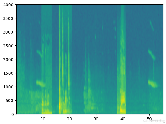
现在您可以听您创建的训练示例,并将其与上面生成的频谱图进行比较。
IPython.display.Audio("train.wav")
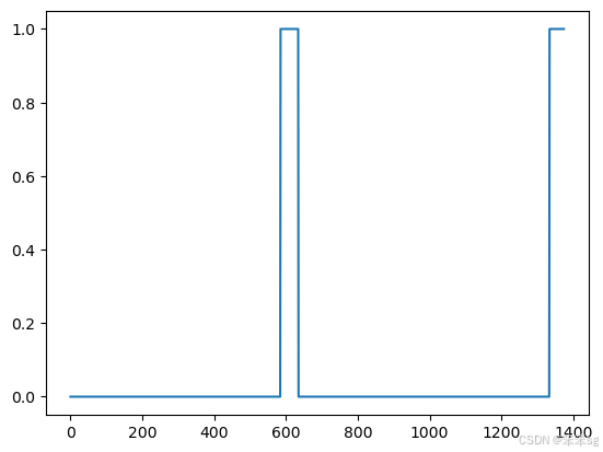
最后,您可以绘制生成的训练示例的相关标签。
plt.plot(y[0])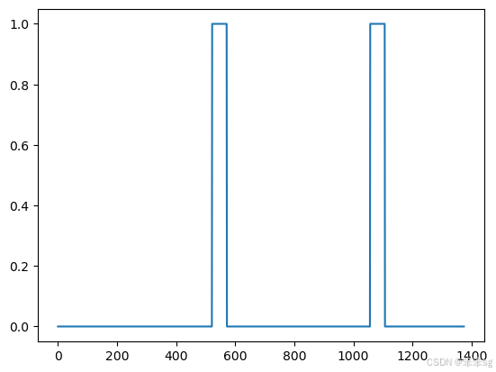
全部训练集
- * 您现在已经实现了生成单个训练示例所需的代码。
- * 我们使用这个过程来生成一个大的训练集。
- * 为了节省时间,我们生成一个较小的32个示例的训练集。
- # START SKIP FOR GRADING
- np.random.seed(4543)
- nsamples = 32
- X = []
- Y = []
- for i in range(0, nsamples):
- if i%10 == 0:
- print(i)
- x, y = create_training_example(backgrounds[i % 2], activates, negatives, Ty)
- X.append(x.swapaxes(0,1))
- Y.append(y.swapaxes(0,1))
- X = np.array(X)
- Y = np.array(Y)
- # END SKIP FOR GRADING
- 0
- (5817, 6471)
- (2497, 4075)
- (9151, 9871)
- (3385, 4963)
- (5426, 6080)
- (2047, 2771)
- (6979, 7385)
- (2647, 3367)
- (1698, 2613)
- (8049, 8957)
- (4926, 5650)
- (5665, 6264)
- (8635, 9359)
- (1288, 3028)
- (4924, 6260)
- (4537, 4891)
- (6835, 7565)
- (1747, 2401)
- (4272, 4626)
- (6573, 7297)
- (7488, 8208)
- (1934, 4325)
- (4585, 6163)
- (8235, 8775)
- Timeouted
- (1750, 2404)
- (9469, 9823)
- (3454, 4369)
- (399, 1129)
- (7335, 8913)
- (2066, 2472)
- (5838, 6492)
- (2884, 4462)
- (1642, 2241)
- (2326, 3050)
- (7830, 8745)
- (5093, 5692)
- 10
- (6266, 6986)
- (7157, 8897)
- (236, 1151)
- (3471, 5211)
- (8859, 9513)
- (1615, 3193)
- (6421, 8812)
- (4022, 5600)
- Timeouted
- (3944, 5522)
- (8843, 9497)
- (90, 668)
- (1378, 2045)
- (7328, 8048)
- (112, 766)
- (6579, 7119)
- (7100, 7640)
- (8605, 9259)
- (4776, 7167)
- (2991, 4731)
- (206, 2597)
- (8109, 9017)
- (7328, 7868)
- Timeouted
- (1742, 2409)
- (4311, 4965)
- (3867, 4224)
- (2713, 3437)
- (5484, 6208)
- (7089, 7756)
- (4882, 5241)
- (8605, 8964)
- 20
- (5746, 8137)
- (7766, 8486)
- (2788, 5179)
- Timeouted
- (6662, 7202)
- (2144, 2695)
- (2132, 2799)
- (8383, 9961)
- (156, 1064)
- (8543, 9197)
- (4702, 5426)
- (6594, 7324)
- (8048, 8963)
- (2261, 2981)
- (6108, 6775)
- (8593, 9247)
- (3330, 4054)
- (4339, 5917)
- (765, 1305)
- (8004, 8410)
- (6125, 7865)
- (1308, 2028)
- (2544, 3268)
- (3912, 5490)
- (2916, 3640)
- (5031, 5939)
- (4099, 4766)
- (777, 1131)
- (2074, 2728)
- 30
- (6855, 7509)
- (5053, 5961)
- (242, 896)
- (1220, 1874)
- (2899, 3305)
- (3467, 4045)
- (4692, 6270)
- (6808, 7532)
- (8937, 9488)

您希望将数据集保存到一个文件中,以便在更实际的环境中稍后加载。我们给你提供以下代码供参考。
- # Save the data for further uses
- # np.save(f'./XY_train/X.npy', X)
- # np.save(f'./XY_train/Y.npy', Y)
- # Load the preprocessed training examples
- # X = np.load("./XY_train/X.npy")
- # Y = np.load("./XY_train/Y.npy")
开发(测试)集
- * 为了测试我们的模型,我们记录了一个包含25个示例的开发集。
- * 虽然我们的训练数据是合成的,但我们希望创建一个与实际输入相同分布的开发集。
- * 因此,我们录制了25个10秒的音频片段,人们说“激活”和其他随机单词,并手工标记。
- * 这遵循课程3“结构化机器学习项目”中描述的原则,我们应该创建开发集尽可能与测试集分布相似
- * 这就是为什么我们的开发团队使用真实音频而不是合成音频的原因。
- # Load preprocessed dev set examples
- X_dev = np.load("./XY_dev/X_dev.npy")
- Y_dev = np.load("./XY_dev/Y_dev.npy")
3.2 触发词检测模型
- * 现在你已经建立了一个数据集,让我们来编写和训练一个触发词检测模型!
- * 模型将使用1-D卷积层、GRU层和dense层。
- * 让我们加载允许你在Keras中使用这些层的包。这可能需要一分钟来加载。
导包
- from tensorflow.keras.callbacks import ModelCheckpoint
- from tensorflow.keras.models import Model, load_model, Sequential
- from tensorflow.keras.layers import Dense, Activation, Dropout, Input, Masking, TimeDistributed, LSTM, Conv1D
- from tensorflow.keras.layers import GRU, Bidirectional, BatchNormalization, Reshape
- from tensorflow.keras.optimizers import Adam
构建模型
我们的目标是建立一个网络,当它检测到触发词时,它将摄取频谱图并输出信号。该网络将使用4层:
* 卷积层
* 两个GRU层
* dense层。
下面是我们将要使用的架构。
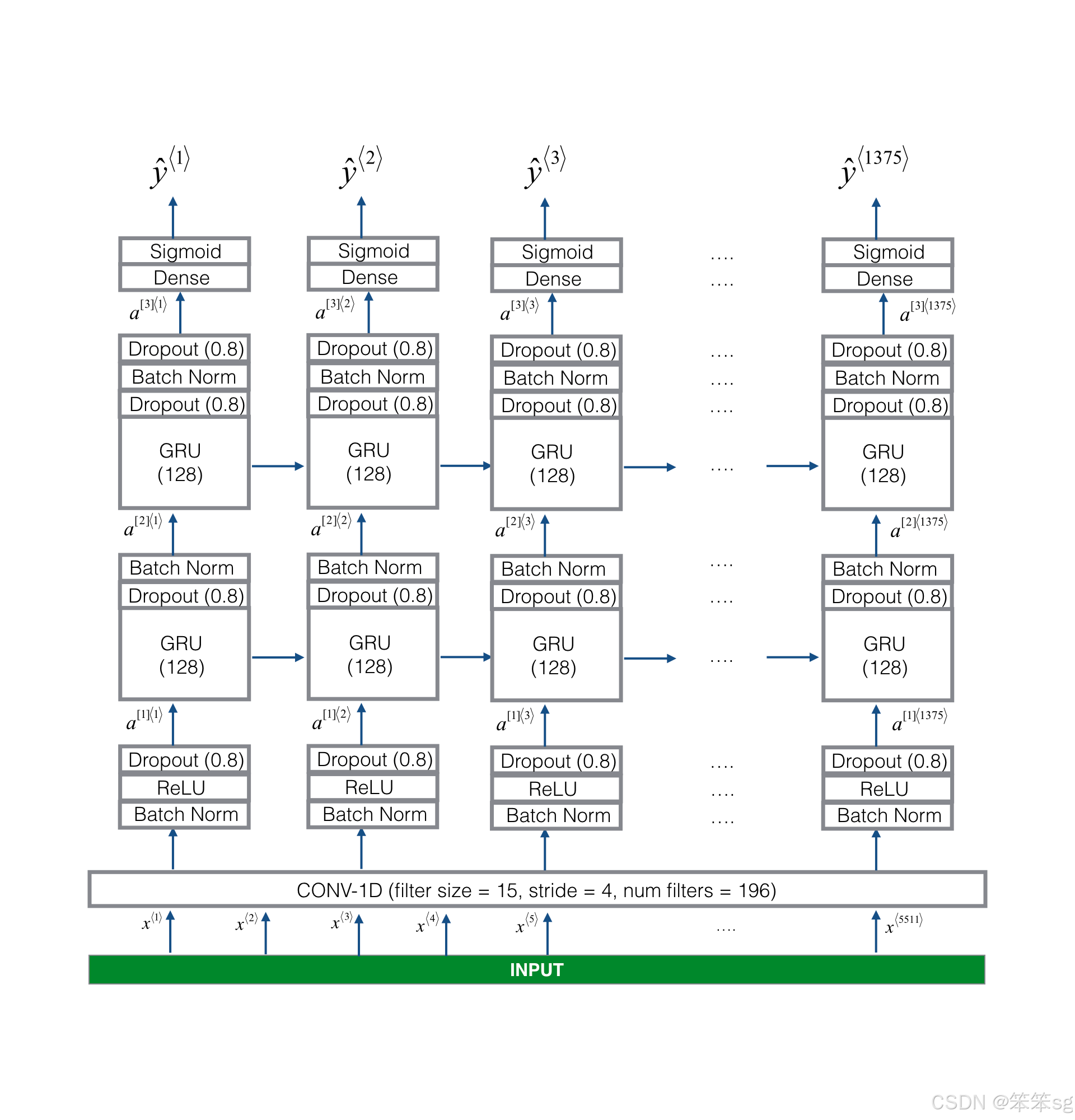
1D 卷积 layer
该模型的一个关键层是1D卷积步骤(接近图3的底部)。
* 输入5511阶跃谱图。每一步都是101个单位的向量。
* 输出1375步进输出
* 该输出由多个层进一步处理以获得最终的
* 这个1D卷积层的作用类似于您在课程4中看到的2D卷积,提取低级特征,然后可能生成较小维度的输出。
* 计算上,一维转换层也有助于加速模型,因为现在GRU只能处理1375个时间步长,而不是5511个时间步长。
GRU, dense and sigmoid
* 两个GRU层从左到右读取输入序列。
* dense层 + sigmod层对
* 因为y是一个二进制值(0或1),我们在最后一层使用sigmoid输出来估计输出为1的可能性,对应于用户刚刚说“activate”。
单向RNN
* 注意,我们使用的是单向RNN,而不是双向RNN。
* 这对于触发词检测非常重要,因为我们希望能够在触发词说出来后几乎立即检测到它。
* 如果我们使用双向RNN,我们将不得不等待整个10秒的音频被记录下来,然后我们才能判断在音频剪辑的第一秒是否说了“激活”。
在下面的模型中,每一层的输入都是前一层的输出。模型的实现可以通过四个步骤来完成。
**Step 1**: CONV层。使用‘ Conv1D() ’来实现这一点,有196个过滤器,过滤器大小为15 (' kernel_size=15 '),步长为4.
**Step 2**: 第一个GRU层。为了生成GRU层,使用128个单元。
**Step 3**: 第二个GRU层。这与第一个GRU层具有相同的规格。
* 接下来是dropout,批处理规范化,然后是另一个dropout。
**Step 4**: 创建一个时间分布的dense层
- # UNQ_C5
- # GRADED FUNCTION: modelf
-
- def modelf(input_shape):
- """
- Function creating the model's graph in Keras.
-
- Argument:
- input_shape -- shape of the model's input data (using Keras conventions)
- Returns:
- model -- Keras model instance
- """
-
- X_input = Input(shape = input_shape)
-
- # Step 1: CONV layer (≈4 lines)
- # Add a Conv1D with 196 units, kernel size of 15 and stride of 4
- X = Conv1D(196, 15, strides=4)(X_input)
- # Batch normalization
- X = BatchNormalization()(X)
- # ReLu activation
- X = Activation('relu')(X)
- # dropout (use 0.8)
- X = Dropout(0.8)(X)
-
- # Step 2: First GRU Layer (≈4 lines)
- # GRU (use 128 units and return the sequences)
- X = GRU(units = 128, return_sequences=True)(X)
- # dropout (use 0.8)
- X = Dropout(0.8)(X)
- # Batch normalization.
- X = BatchNormalization()(X)
-
- # Step 3: Second GRU Layer (≈4 lines)
- # GRU (use 128 units and return the sequences)
- X = GRU(units = 128, return_sequences=True)(X)
- # dropout (use 0.8)
- X = Dropout(0.8)(X)
- # Batch normalization
- X = BatchNormalization()(X)
- # dropout (use 0.8)
- X = Dropout(0.8)(X)
-
- # Step 4: Time-distributed dense layer (≈1 line)
- # TimeDistributed with sigmoid activation
- X = TimeDistributed(Dense(1, activation = "sigmoid"))(X)
-
- model = Model(inputs = X_input, outputs = X)
-
- return model
- # UNIT TEST
- from test_utils import *
-
- def modelf_test(target):
- Tx = 5511
- n_freq = 101
- model = target(input_shape = (Tx, n_freq))
- expected_model = [['InputLayer', [(None, 5511, 101)], 0],
- ['Conv1D', (None, 1375, 196), 297136, 'valid', 'linear', (4,), (15,), 'GlorotUniform'],
- ['BatchNormalization', (None, 1375, 196), 784],
- ['Activation', (None, 1375, 196), 0],
- ['Dropout', (None, 1375, 196), 0, 0.8],
- ['GRU', (None, 1375, 128), 125184, True],
- ['Dropout', (None, 1375, 128), 0, 0.8],
- ['BatchNormalization', (None, 1375, 128), 512],
- ['GRU', (None, 1375, 128), 99072, True],
- ['Dropout', (None, 1375, 128), 0, 0.8],
- ['BatchNormalization', (None, 1375, 128), 512],
- ['Dropout', (None, 1375, 128), 0, 0.8],
- ['TimeDistributed', (None, 1375, 1), 129, 'sigmoid']]
- comparator(summary(model), expected_model)
-
-
- modelf_test(modelf)
All tests passed!
model = modelf(input_shape = (Tx, n_freq))让我们打印模型摘要以跟踪形状。
model.summary()- Model: "model_1"
- _________________________________________________________________
- Layer (type) Output Shape Param #
- =================================================================
- input_2 (InputLayer) [(None, 5511, 101)] 0
- _________________________________________________________________
- conv1d_1 (Conv1D) (None, 1375, 196) 297136
- _________________________________________________________________
- batch_normalization_3 (Batch (None, 1375, 196) 784
- _________________________________________________________________
- activation_1 (Activation) (None, 1375, 196) 0
- _________________________________________________________________
- dropout_4 (Dropout) (None, 1375, 196) 0
- _________________________________________________________________
- gru_2 (GRU) (None, 1375, 128) 125184
- _________________________________________________________________
- dropout_5 (Dropout) (None, 1375, 128) 0
- _________________________________________________________________
- batch_normalization_4 (Batch (None, 1375, 128) 512
- _________________________________________________________________
- gru_3 (GRU) (None, 1375, 128) 99072
- _________________________________________________________________
- dropout_6 (Dropout) (None, 1375, 128) 0
- _________________________________________________________________
- batch_normalization_5 (Batch (None, 1375, 128) 512
- _________________________________________________________________
- dropout_7 (Dropout) (None, 1375, 128) 0
- _________________________________________________________________
- time_distributed_1 (TimeDist (None, 1375, 1) 129
- =================================================================
- Total params: 523,329
- Trainable params: 522,425
- Non-trainable params: 904
- _________________________________________________________________
网络的输出形状为(None, 1375,1),而输入形状为(None, 5511,101)。Conv1D将步骤数从5511减少到1375。
训练模型
- * 触发词检测需要很长时间来训练。
- * 为了节省时间,我们已经使用你上面构建的架构在GPU上训练了大约3个小时的模型,以及大约4000个示例的大型训练集。
- * 让我们加载模型。
- from tensorflow.keras.models import model_from_json
-
- json_file = open('./models/model.json', 'r')
- loaded_model_json = json_file.read()
- json_file.close()
- model = model_from_json(loaded_model_json)
- model.load_weights('./models/model.h5')
如果要对预训练模型进行微调,那么阻塞所有批处理归一化层的权重是很重要的。如果您打算从头开始训练一个新模型,请跳过下一个单元格。
- model.layers[2].trainable = False
- model.layers[7].trainable = False
- model.layers[10].trainable = False
您可以使用Adam优化器和二元交叉熵损失进一步训练模型,如下所示。这将运行得很快,因为我们只训练了两个epoch,并且训练集很小,只有32个样本。
- opt = Adam(lr=1e-6, beta_1=0.9, beta_2=0.999)
- model.compile(loss='binary_crossentropy', optimizer=opt, metrics=["accuracy"])
model.fit(X, Y, batch_size = 16, epochs=1)2/2 [==============================] - 8s 176ms/step - loss: 0.4388 - accuracy: 0.8713
测试模型
最后,让我们看看模型在开发集上的表现。
- loss, acc, = model.evaluate(X_dev, Y_dev)
- print("Dev set accuracy = ", acc)
1/1 [==============================] - 1s 883ms/step - loss: 0.1883 - accuracy: 0.9238
Dev set accuracy = 0.9237818121910095
看起来很不错!
- * 然而,准确性并不是这项任务的重要指标
- * 由于标签严重偏向于0,因此只输出0的神经网络将获得略高于90%的准确率。
- * 我们可以定义更有用的指标,如F1分数或Precision/Recall。
- * 这里我们就不讨论这个了,我们来看看这个模型是如何预测的。
3.3 做预测
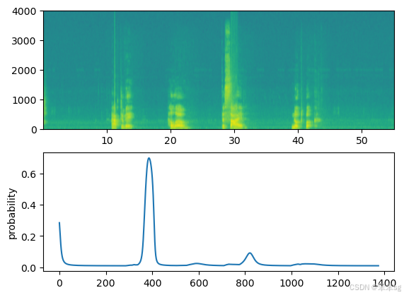
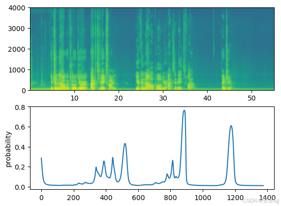
现在您已经为触发词检测构建了一个工作模型,让我们使用它来进行预测。这个代码片段通过网络运行音频(保存在wav文件中)
- def detect_triggerword(filename):
- plt.subplot(2, 1, 1)
-
- # Correct the amplitude of the input file before prediction
- audio_clip = AudioSegment.from_wav(filename)
- audio_clip = match_target_amplitude(audio_clip, -20.0)
- file_handle = audio_clip.export("tmp.wav", format="wav")
- filename = "tmp.wav"
-
- x = graph_spectrogram(filename)
- # the spectrogram outputs (freqs, Tx) and we want (Tx, freqs) to input into the model
- x = x.swapaxes(0,1)
- x = np.expand_dims(x, axis=0)
- predictions = model.predict(x)
-
- plt.subplot(2, 1, 2)
- plt.plot(predictions[0,:,0])
- plt.ylabel('probability')
- plt.show()
- return predictions
插入一个报时以确认“activate”的出现
- *一旦你估算出在每个输出步骤中检测到单词“activate”的概率,你就可以在概率高于某个阈值时触发“chiming”声音播放。
- * 可能在“activate”之后连续许多值接近1,但我们只想发出一次报时。
- * 因此,我们将每75个输出步骤最多插入一次编钟声音。
- * 这将有助于防止我们为一个“activate”实例插入两个编钟。
- * 这与计算机视觉的非最大抑制作用类似。
- chime_file = "audio_examples/chime.wav"
- def chime_on_activate(filename, predictions, threshold):
- audio_clip = AudioSegment.from_wav(filename)
- chime = AudioSegment.from_wav(chime_file)
- Ty = predictions.shape[1]
- # Step 1: Initialize the number of consecutive output steps to 0
- consecutive_timesteps = 0
- # Step 2: Loop over the output steps in the y
- for i in range(Ty):
- # Step 3: Increment consecutive output steps
- consecutive_timesteps += 1
- # Step 4: If prediction is higher than the threshold and more than 20 consecutive output steps have passed
- if consecutive_timesteps > 20:
- # Step 5: Superpose audio and background using pydub
- audio_clip = audio_clip.overlay(chime, position = ((i / Ty) * audio_clip.duration_seconds) * 1000)
- # Step 6: Reset consecutive output steps to 0
- consecutive_timesteps = 0
- # if amplitude is smaller than the threshold reset the consecutive_timesteps counter
- if predictions[0, i, 0] < threshold:
- consecutive_timesteps = 0
-
- audio_clip.export("chime_output.wav", format='wav')
开发示例测试
让我们来探索我们的模型如何处理来自开发集的两个未见过的音频剪辑。让我们先来听两个开发集的剪辑。
IPython.display.Audio("./raw_data/dev/1.wav")![]()
现在让我们在这些音频片段上运行模型,看看它是否在“activate”之后添加了一个编钟!
- filename = "./raw_data/dev/1.wav"
- prediction = detect_triggerword(filename)
- chime_on_activate(filename, prediction, 0.5)
- IPython.display.Audio("./chime_output.wav")
![]()
这是你应该记住的:
- 数据合成是为语音问题创建大型训练集的有效方法,特别是触发词检测。
- 在将音频数据传递给RNN, GRU或LSTM之前,使用频谱图和可选的1D转换层是常见的预处理步骤。
- 端到端深度学习方法可用于构建非常有效的触发词检测系统。
3.4 试试你自己的例子!
您可以在自己的音频剪辑上尝试您的模型!
- * 录制一段10秒的你说“激活”和其他随机单词的音频片段,并将其上传到Coursera中心,命名为“myaudio.wav”。
- * 请确保以wav文件上传音频。
- * 如果你的音频是以不同的格式录制的(如mp3),你可以在网上找到免费的软件将其转换为wav。
- * 如果你的音频记录不是10秒,下面的代码将根据需要修剪或填充它,使它成为10秒。
- # Preprocess the audio to the correct format
- def preprocess_audio(filename):
- # Trim or pad audio segment to 10000ms
- padding = AudioSegment.silent(duration=10000)
- segment = AudioSegment.from_wav(filename)[:10000]
- segment = padding.overlay(segment)
- # Set frame rate to 44100
- segment = segment.set_frame_rate(44100)
- # Export as wav
- segment.export(filename, format='wav')
将音频文件上传到Coursera后,将文件的路径放在下面的变量中。
your_filename = "audio_examples/my_audio.wav"- preprocess_audio(your_filename)
- IPython.display.Audio(your_filename) # listen to the audio you uploaded
![]()
最后,使用这个模型来预测你在10秒的音频片段中说激活的时间,并触发一个编钟。如果没有适当地添加蜂鸣声,请尝试调整chime_threshold。
- chime_threshold = 0.3 # 触发蜂鸣器的阈值
- prediction = detect_triggerword(your_filename)
- chime_on_activate(your_filename, prediction, chime_threshold)
- IPython.display.Audio("./chime_output.wav")
![]()
评论记录:
回复评论: